1.

Introduction

We define ocean color as the spectral distribution of reflected visible solar radiation upwelling from beneath the ocean surface. Variations in this water-leaving remote sensing reflectance distribution, $\mathrm{Rrs}(\lambda )$, the ratio of radiance emerging from beneath the ocean surface to the solar irradiance reaching the ocean surface, are governed by the optically active biological and chemical constituents of the upper ocean through their absorption and scattering properties. A primary driver for variations in ocean color is the concentration of the phytoplankton pigment chlorophyll $a$ ($\mathrm{C}a$; $\mathrm{mg}{\mathrm{m}}^{-3}$), and bio-optical algorithms have been developed that relate measurements of $\mathrm{Rrs}(\lambda )$ to $\mathrm{C}a$ that provide a proxy for phytoplankton biomass.¹ As marine phytoplankton account for roughly half the net primary productivity on Earth,² ocean color measurements are critical to our understanding of planetary health and the global carbon cycle. Other bio-optical and biogeochemical properties that can be inferred from $\mathrm{Rrs}(\lambda )$ include spectral absorption by colored dissolved organic matter (CDOM), concentrations of total suspended sediments, measurements of water clarity, such as marine diffuse attenuation coefficient and euphotic depth, and the presence of harmful algal blooms. Ocean color, thus, also provides a valuable tool for monitoring water quality and changes in the marine environment that can directly impact human health and commerce, especially in coastal areas and near lakes and inland waterways, where much of the human population resides.

Landsat-8 was launched into a sun-synchronous polar orbit on February 11, 2013, carrying with it the Operational Land Imager³ (OLI, Table 1). Prelaunch simulations based on radiometric performance specifications demonstrated that the sensor, while primarily designed for land applications, has the potential to provide useful measurements of aquatic environments, including the separation and quantification of $\mathrm{C}a$, CDOM, and suspended sediments in the water column.^4,5 A significant advantage of OLI over existing global ocean color capable missions is the 30 m spatial resolution, which is more than an order of magnitude higher than NASA’s Moderate Resolution Imaging Spectroradiometer⁶ (MODIS) currently operating from the Aqua spacecraft (MODISA) and the Sea-viewing Wide Field-of-View Sensor⁷ (SeaWiFS) that operated from 1997 to 2010. Increased spatial resolution is of particular benefit in studying heterogeneous coastal and inland waters, where the typical 1 km resolution of existing global sensors cannot resolve the fine spatial structure of the water constituents or separate water from land near coasts and in narrow rivers and bays. Thus, OLI on Landsat-8 has the potential to make a valuable contribution to ocean color science and environmental monitoring capabilities for aquatic ecosystems, especially in coastal environments and inland waters.

Table 1

Landsat-8 Operational Land Imager (OLI) mission and sensor characteristics.

The measurement of ocean color from spaceborne instruments is challenging because the water-leaving signal is only a small fraction of the total signal reflected by the Earth into the sensor field of view. Approximately 90% of the visible radiation observed by Earth-viewing satellite sensors is sunlight reflected by air molecules and aerosols in the atmosphere. The removal of this atmospheric signal to retrieve $\mathrm{Rrs}(\lambda )$ is referred to as atmospheric correction. NASA’s Ocean Biology Processing Group distributes a software package called the SeaWiFS Data Analysis System (SeaDAS)⁸ that provides the research community with a standardized tool for the production, display, and analysis of ocean color products from a host of Earth-viewing multispectral radiometers. SeaDAS contains within it the multisensor level 1 to level 2 generator (l2gen) that can read level 1 observed top-of-atmosphere (TOA) radiances from a variety of sensors, perform the atmospheric correction process, and retrieve $\mathrm{Rrs}(\lambda )$ and various derived geophysical properties. The l2gen code can be adapted to work with any sensor that has a sufficient set of spectral bands covering the blue to green region of the visible spectrum (i.e., 400 to 600 nm), with at least two bands in the near-infrared (NIR) to shortwave IR (SWIR) to support the atmospheric correction.

OLI has a sufficient set of spectral bands for ocean color retrievals (Table 2). Precise atmospheric correction also requires that the radiometric performance (signal relative to noise) and digital resolution (number of bits available to encode the observed radiance) are sufficiently high to detect the relatively small water-leaving radiance signal above the sensor noise. In the sections that follow, we assess the radiometric performance of the OLI instrument for ocean color applications and detail the adaptation of l2gen in SeaDAS to support OLI atmospheric correction. We also present results of an initial system-level vicarious calibration, where match-ups to in situ radiometry are used to refine the $\mathrm{Rrs}(\lambda )$ retrieval performance of the combined OLI instrument and atmospheric correction process. Finally, we show some results of ocean color retrieval over the coastal and inland waters of Chesapeake Bay and compare them with coincident MODISA retrievals and in situ measurements.

Table 2

Landsat-8 OLI spectral bands and signal-to-noise ratios (SNR).

2.

Data and Sensor Characteristics

OLI data are freely available for direct download or bulk ordering from the website of the U.S. Geological Survey (USGS), which operates the Landsat-8 mission. The observed TOA radiances (Level-1T) are provided in GeoTIFF format, with each spectral band in a separate file that has been mapped to a common Universal Transverse Mercator (UTM) projection. The full suite of spectral band files are packaged into a compressed tape archive (tar) file that also includes a Landsat Metadata (MTL) file in text form containing scene-specific time and location information.

OLI is a push-broom design with 14 separate detector assemblies aligned across the orbit track to create a swath of $\sim 185\mathrm{km}$ width or $\sim 7000\mathrm{pixels}$. The 14 detector assemblies alternate between slightly forward-pointing and slightly aft-pointing, and the spectral bands are aligned along track such that the amount of forward and aft pointing varies by band.⁹ The effect is that each spectral band views the same point on the Earth at a slightly different time and with a slightly different atmospheric path (characterized by sensor zenith and azimuth angles), and the path angles alternate fore and aft across the swath. Cross-track variations in geolocation and spectral band registration are effectively removed by mapping of the native observations to a common UTM projection in the Level-1T product, but the TOA radiances retain characteristics of their observational geometry that must be considered in ocean color retrieval.

Accurate atmospheric correction over the comparatively dark ocean requires precise knowledge of the solar and viewing path geometry. For the bands of interest to ocean color, the spectral variation in view zenith and azimuth angle is on the order of 0.2 deg and can be safely ignored, but mean variation in solar and view zenith and azimuth across the swath must be known, and the fore and aft variation between detector assemblies must be accounted for or significant along-track banding artifacts due to atmospheric correction error will be evident in the $\mathrm{Rrs}(\lambda )$ retrievals. The Level-1T data product does not include this additional geometry information, but USGS has developed software to estimate it for each scene pixel for each sensor band from information contained in the scene MTL file. This USGS software has been incorporated into SeaDAS/l2gen to automatically produce band-averaged solar and viewing geometry sufficient for ocean color retrieval.

Accurate atmospheric correction and $\mathrm{Rrs}(\lambda )$ retrieval also requires a sensor with sufficient signal-to-noise ratio (SNR) over ocean waters to detect and differentiate the water-leaving signal. For relatively clear, low-productivity waters typical of the open oceans, an inadequate SNR will contribute to a large relative error in $\mathrm{Rrs}(\lambda )$ in the green and red spectral range, where pure water absorption and minimal particle scattering contributions produce a comparatively small water-leaving reflectance. In contrast, turbid coastal and inland waters with high sediment loads present less of a challenge in the green and red due to the high particle scattering contributions, but for these waters, a low SNR will often lead to a high relative error in Rrs(443) retrievals, as high absorption by $\mathrm{C}a$ and CDOM depresses the water-leaving signal in the blue. Finally, depending on the atmospheric correction approach, low SNR in the NIR or SWIR channels can contribute to noise and systematic bias across the visible spectral range, due to error in estimating the aerosol contribution to the observed signal.¹⁰

OLI is the most advanced radiometer ever flown on a Landsat platform, with SNRs roughly an order of magnitude higher than the predecessor Enhanced Thematic Mapper Plus ($\mathrm{ETM}+$) instrument of Landsat-7 and 12-bit rather than 8-bit digital resolution.¹¹ The SNRs reported for OLI or $\mathrm{ETM}+$, however, are based on radiances typical of land observations. To assess potential OLI performance over oceans, the sensor noise model¹¹ was applied to typical radiances (Ltyp) interpolated from values reported in Ref. 10, which were themselves based on average radiances observed by MODISA over ocean targets at $\sim 45\mathrm{deg}$ solar zenith angle. Using these Ltyps, the derived OLI SNRs (Table 2) can be directly compared to those of SeaWiFS and MODISA, as also reported in Ref. 10. In general, the OLI SNRs are lower than those of SeaWiFS or MODISA, but visible-band SNRs are within 50% of SeaWiFS (specified or observed), and OLI SWIR-band SNRs are equally similar to comparable MODISA SWIR bands. The biggest discrepancy is at 865 nm, where the OLI SNR of 67 is substantially lower than the SeaWiFS specification (287), but is still within a factor of 3 of the observed SeaWiFS SNR.¹⁰ It should also be recognized that OLI observations are at a much higher spatial resolution than SeaWiFS or MODIS, and spatial averaging over a few pixels could significantly increase the SNRs, as demonstrated in Ref. 5. Similar SNR results have been previously reported by Pahlevan et al., based on statistical analysis of uniform OLI scenes over oceans.¹² Given the SNR equivalency with successful heritage ocean color sensors, the OLI radiometric performance appears sufficient for many ocean color applications.

For context, the SNRs of $\mathrm{ETM}+$ are also reported in Table 2 for equivalent spectral bands using the same Ltyps and the high-gain noise model developed for the instrument.¹³ Results confirm the significant advancement of the OLI radiometric performance over ETM+. The numbers also suggest that the NIR and SWIR bands of $\mathrm{ETM}+$ are effectively unusable for the atmospheric correction approach that we propose here for OLI, as noise in the NIR channel is equivalent to 10% of the signal and noise in the longest SWIR spectral band actually exceeds the typical radiance over oceans.

3.

Processing Approach

3.3.

Vicarious Calibration

Given the stringent accuracy requirements of satellite ocean color retrievals for both the instrument calibration and the atmospheric correction algorithm, an additional vicarious calibration was derived. This temporally independent but wavelength-specific calibration minimizes residual bias and enhances spectral consistency of the $\text{sensor}+\text{algorithm}$ system under idealized conditions.³³ The primary vicarious calibration source for all NASA ocean color missions is the marine optical buoy (MOBY)³⁴ near Lanai, Hawaii, which has been continuously operated by NOAA since 1996. A time-series of all OLI scenes covering the Lanai region was collected and filtered to find cases of relatively clear, cloud-free atmospheric conditions and negligible Sun glint. The full screening and averaging process is detailed in Ref. 33. Two scenes were found to pass all screening criteria (Fig. 1), and vicarious calibration gains were derived for each (Table 4). For this initial evaluation, the calibration of the atmospheric correction bands at 865 and 2201 nm was not altered.

Fig. 1

Operational Land Imager (OLI) images over Lanai, Hawaii, on (a) January 9, 2014, and (b) February 10, 2014, showing location of the NOAA marine optical buoy (MOBY). Colocated data from MOBY and OLI on these dates were used in the OLI vicarious calibration.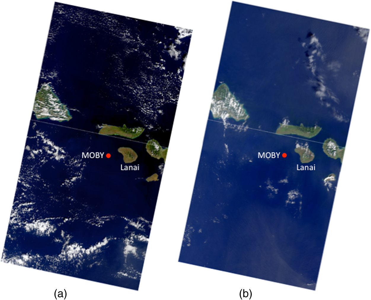

Table 4

OLI vicarious calibration gains.

	Band 1	Band 2	Band 3	Band 4	Band 5	Band 6	Band 7
Jan 09, 2014	1.01932	1.04007	1.00720	1.01239	1.0	0.94364	1.0
Feb 10, 2014	1.01771	1.04022	1.00734	1.01740	1.0	0.91266	1.0
Avg. gain	1.0185	1.0401	1.0073	1.0149	1.0	0.9282	1.0

The change in color between the two images in Fig. 1, which were collected about one month apart, is due to the difference in solar geometry and a change in the aerosol conditions. Notably, the vicarious calibration was highly consistent between the two scenes, suggesting that the atmospheric modeling compensated well for the changes observed between the two dates. The average vicarious gain in each band (Table 4) was implemented for all subsequent processing.

4.

Results and Discussion

The atmospheric correction approach discussed above and the vicarious calibration from Table 4 were applied to a series of OLI Level-1T scenes collected over the Chesapeake Bay region. Rrs(443) and Rrs(561) retrievals from a partial OLI scene on September 5, 2013, focusing on the mouth of the Bay from Cape Charles to Virginia Beach and the inlets of the James, York, and Rappahannock Rivers, show good agreement with coincident Rrs(443) and Rrs(547) retrievals from MODISA (Fig. 2). The MODISA data were collected on the same day and processed with the same atmospheric correction approach, but using the sensor-specific spectral response functions and a sensor-specific vicarious calibration. Also evident in this comparison is the enhanced information content that 30 m spatial resolution provides relative to the $>1\mathrm{km}$ resolution of MODIS, allowing observations closer to the coasts and further into rivers and bays, and better resolving the spatial variability of optically active constituents within the water bodies.

Fig. 2

Images of water-leaving reflectances, Rrs, for OLI bands at (a) 443 nm and (b) 561 nm, retrieved over Chesapeake Bay on 5 September 2013, with MODIS Aqua retrievals of (c) 443 nm and (d) 547 nm shown for comparison. The MODIS data was collected on the same day, about 3 h later, and $\mathrm{Rrs}(\lambda )$ was retrieved using standard NASA ocean color processing in SeaDAS.

The $\mathrm{Rrs}(\lambda )$ retrievals from OLI were applied to the empirical $\mathrm{C}a$ algorithm and compared with the equivalent product from MODISA (Fig. 3). In general, OLI $\mathrm{C}a$ retrievals for this day over the main stem of the lower Chesapeake Bay region are lower than those retrieved from MODISA. Assuming MODISA is correct, this would suggest that the Rrs(443) or Rrs(482) retrievals are too high relative to Rrs(561), i.e., the spectral dependence is biased toward the blue, which may be due to uncertainty in the vicarious calibration or error in the aerosol retrieval. Unfortunately, there is also considerable uncertainty in the MODISA instrument calibration in the latter period of the mission,³⁵ so interpretation of this result as error in the OLI retrieval should be made with caution.

Fig. 3

Images of chlorophyll $a$ concentration retrieved from OLI and MODIS Aqua over Chesapeake Bay on September 5, 2013. The MODIS data were collected on the same day, about 3 h later. The chlorophyll $a$ concentration was retrieved using standard NASA ocean color processing in SeaDAS.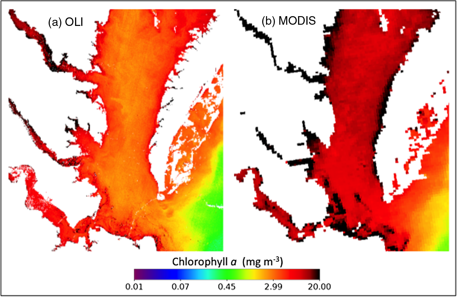

The spatial detail of the OLI ocean color retrievals is well illustrated in Fig. 4, where the red, green, and blue $\mathrm{Rrs}(\lambda )$ products at 655, 561, and 443 nm, respectively, have been combined into a quasi true-color image. This image, collected on February 28, 2014, shows striking detail of the presence of suspended sediments and other optically active biogeochemical constituents around coastal landforms and where rivers enter the Bay. Sediment plumes, for example, are clearly evident offshore of the Potomac and Rappahannock Rivers despite February 2014 being an average year with regard to streamflow³⁶ and free of any notable winter storms. The barrier islands between Hills Bay and Winter Harbor (between the Rappahannock and York Rivers) show significant suspended sediment loads, likely either from advective oceanward transport from the Rappahannock River or from wind-driven resuspension. Likewise, some of the shallowest areas of Chesapeake Bay, e.g., east of Smith and Tangier Islands, show substantial (re)suspended sediment loads. The high spatial resolution and relatively high SNR of OLI makes it possible to resolve the spatial structure of these estuarine features.

Fig. 4

Three-band water-leaving reflectance, $\mathrm{Rrs}(\lambda )$, composite image over the mouth of Chesapeake Bay showing detailed distribution patterns of sediments and colored organic matter that can be retrieved from OLI using standard NASA ocean color processing in SeaDAS. The composite was generated using the red, green, and blue reflectances at 655, 561, and 443 nm, respectively.

To further demonstrate the advantage that OLI spatial resolution provides over MODIS, Fig. 5 shows the same $\mathrm{Rrs}(\lambda )$ composite zoomed in to the mouth of the Potomac River, with MODISA scan-pixel boundaries for the same day overlaid. The OLI images show fine detail in ocean color that cannot be resolved by the larger MODIS pixels. OLI, thus, provides an unprecedented opportunity to directly observe this MODIS subpixel variability in suspended sediments and organic material, which can provide valuable insight into uncertainties in MODIS ocean color retrievals³⁷ and improved understanding of differences observed in validation match-ups to localized in situ measurements.

Fig. 5

Three-band water-leaving reflectance composite image from OLI at the location where the Potomac River enters Chesapeake Bay. MODIS Aqua scan pixel boundaries for the same date are overlaid to demonstrate the subpixel variability revealed by the higher spatial resolution of OLI.

$\mathrm{Rrs}(\lambda )$ composite images and $\mathrm{C}a$ retrievals were generated for five scenes obtained over Chesapeake Bay between September 2013 and April 2014 (Fig. 6). The general similarity of the ocean color images suggests good temporal stability of the OLI calibration and good performance of the atmospheric correction algorithm over a wide range of solar geometries. These five scenes represent all available relatively cloud-free, glint-free scenes of Chesapeake Bay currently available from OLI, thus, Fig. 6 provides an indication of the frequency at which a mid-latitude location may be monitored with OLI, considering cloudy days and the 16-day repeat cycle of Landsat-8. Due to the solar and viewing path geometry, OLI observations between late spring and early fall over mid-latitude oceans of the northern hemisphere are heavily contaminated by specular reflection of the Sun by the sea surface. Our algorithm attempts to remove this Sun glint contribution,²³ but residual error in high glint conditions (glint-favorable geometries) can dominate the subsurface signal and substantially degrade $\mathrm{Rrs}(\lambda )$ retrieval quality, or cause the retrieval process to fail completely due to contamination of the aerosol selection bands.

Fig. 6

OLI true-color images, $\mathrm{Rrs}(\lambda )$ composite images, and chlorophyll $a$ retrievals from all available clear scenes over Chesapeake Bay.

For a more quantitative assessment of OLI ocean color retrieval performance, the distribution of $\mathrm{C}a$ and $\mathrm{Rrs}(\lambda )$ over Chesapeake Bay was compared to same-day retrievals from MODISA. Following Werdell et al.,³⁸ data from the five scenes of Fig. 6 were geographically stratified into lower and middle Bay regions to produce the regional frequency distributions of Fig. 7. Also shown is the mean distribution from SeaWiFS over the mission lifespan (1997 to 2010), to provide additional context on expected range of values. Results show relatively good agreement between OLI and MODISA $\mathrm{Rrs}(\lambda )$ distributions, especially in the green [i.e., Rrs(561) of OLI compared with Rrs(547) of MODISA), and both sensors are in good agreement with the SeaWiFS mission mean. Agreement is not quite as good for the bluest band, with OLI Rrs(443) being elevated relative to MODISA Rrs(443). This gives rise to a larger blue/green ratio from OLI, and thus lower $\mathrm{C}a$ retrievals relative to MODISA, as previously presented in Fig. 3. These differences may simply be the result of uncertainty in the OLI vicarious calibration derived from just two MOBY measurements, or the as yet uncorrected atmospheric correction bands, but the discrepancy may also arise from error in MODISA retrievals due to degradation in temporal calibration,³⁵ or possibly contamination by stray light where the high contrast in the NIR between dark water and adjacent bright land can lead to overestimation of aerosol contributions and, thus, underestimation of Rrs(443) for MODISA.³⁹ Instrumental stray light contamination has been found to be minimal in OLI.¹¹

Fig. 7

Comparison of OLI, MODIS Aqua, and Sea-viewing Wide Field-of-View Sensor (SeaWiFS) chlorophyll $a$ and $\mathrm{Rrs}(\lambda )$ retrieval distributions in the middle and lower Chesapeake Bay, following Ref. 38. OLI (red) and MODIS (blue) data were collected over the same five dates shown in Fig. 6. SeaWiFS data (gray shaded) show the average over the mission lifetime (1997 to 2010). In situ chlorophyll $a$ measurements shown in black were collected within the same region at regular spatial and temporal sampling intervals over the period from 1984 to 2010 (Chesapeake Bay Program⁴⁰).

The $\mathrm{C}a$ values from OLI and MODISA in the middle Bay do straddle the range of values measured over previous years by SeaWiFS, and the OLI retrievals of $\mathrm{C}a$ in the lower Bay are in very good agreement with expectation based on historical SeaWiFS retrievals. Also shown in Fig. 7 is the distribution of in situ $\mathrm{C}a$ measurements collected at regular spatial and temporal sampling intervals over a 26-year period from 1984 to 2010,⁴⁰ showing that these OLI $\mathrm{C}a$ retrievals fall within the range of values expected from historical field observations.

5.

Conclusions

While there is a long history of efforts to utilize earlier Landsat missions and associated sensors, such as $\mathrm{ETM}+$ on Landsat-7, for water quality assessment of coastal and inland waters,^41,42 the comparatively poor radiometric performance (demonstrated here by the much lower SNR of $\mathrm{ETM}+$ relative to OLI) has largely restricted these efforts to retrieval of suspended sediments only, where high backscatter provides a sufficiently robust signal to compensate for sensor noise and digitization error. These past efforts also generally relied on minimal atmospheric correction or simplifying assumptions, such as attributing the Rayleigh-subtracted reflectance in the SWIR as $\mathrm{glint}+\mathrm{aerosol}$ reflectance and removing this from the visible bands by assuming a flat spectral dependence.⁴² Based on an analysis of the sensor signal to noise for typical ocean radiances, and comparison with successful heritage ocean color sensors, we conclude that OLI has the requisite spectral bands and sufficient radiometric performance to support the standard atmospheric correction approach used for NASA’s global ocean color missions, including determination and removal of aerosol contributions based on realistic aerosol models and OLI observations in the NIR and SWIR, and to enable the quantitative retrieval of water column constituents from the derived spectral water-leaving reflectance distributions.

NASA’s standard atmospheric correction and ocean color retrieval algorithms, as originally developed for SeaWiFS and MODIS, were modified to support the OLI data format and sensor spectral characteristics, and an initial vicarious calibration was performed. Evaluation of OLI ocean color retrieval over a time-series of Chesapeake Bay scenes demonstrated relatively good agreement with other ocean color sensors and with historical field measurements in the region. The observed agreement may further improve as instrument temporal calibration is refined and additional MOBY measurements are incorporated to reduce uncertainty in the OLI vicarious calibration, but these initial results demonstrate that OLI can be a valuable tool for ocean color science and environmental monitoring applications.

We showed that a primary advantage of OLI over heritage global ocean color imagers, such as MODIS, is the much higher spatial resolution that allows resolving the fine-scale distribution of suspended sediments and bio-optical water constituents in coastal and estuarine environments. A limitation of OLI for routine observation and monitoring of these dynamic regions is the narrow swath and relatively infrequent 16-day repeat cycle, coupled with observational losses due to cloud cover and the confounding effects of Sun glint. Use of high spatial resolution OLI in combination with the more frequent (one-to-two day) repeat cycle of existing wide-swath, moderate-resolution global imagers can, thus, provide complementary observations to better understand and monitor spatial and temporal ecosystem dynamics in nearshore environments, as well as for understanding the inherent uncertainty in moderate-resolution sensors due to unresolved subpixel variability.

The higher spatial resolution of OLI does lead to additional challenges relative to moderate-resolution sensors. For example, our algorithm for Sun glint correction is based on a statistical model developed by Cox and Munk,⁴³ which provides the probability distribution function for surface facets being oriented in the specular direction, parameterized as a function of wind speed. The validity of this statistical relationship degrades as resolution increases and individual wave orientations are resolved, as is the case for OLI. Alternative methods based on observed radiometry have been investigated for higher spatial resolution sensors (see Ref. 44 for a review), and we suggest that development of an improved glint correction approach for OLI should be a focus of future work.

Another challenge for quantitative ocean color measurement in nearshore environments, which has not been addressed here, is the adjacency effect wherein observations of dark water pixels are contaminated by light reflected from adjacent bright land surfaces that is subsequently scattered into the sensor field of view by the atmosphere.^45–47 The adjacency effect impacts both moderate and higher spatial resolution ocean color observations, as the influence of land reflectance on water observations can extend over 20 km from the coast,⁴⁶ but the impact increases with proximity to the bright reflecting source, thus, it is a still greater concern for the higher-resolution OLI observations that extend closer to the land/water boundary, and particularly for observations in narrow rivers and small lakes that are surrounded by land. More work is needed to assess the impact of atmospheric adjacency and develop a viable correction strategy to mitigate this effect.

Support for atmospheric correction and ocean color product retrieval from OLI has now been incorporated into l2gen, a component of NASA’s open-source SeaDAS software package that is made freely available to the research and applications community for the processing, visualization, and analysis of satellite radiometry from a host of ocean color capable sensors. In addition to the processing algorithms described here, SeaDAS provides many alternative methods and variations that are applicable to OLI, as well as a wide range of derived product algorithms beyond $\mathrm{C}a$. For atmospheric correction, for example, use of alternate band pairs for aerosol selection, fixed aerosol type based on in situ knowledge, and alternate methods for resolving the water-leaving radiance contribution in the NIR to SWIR can now be evaluated.^17,18 Additional products that can be derived from the retrieved Rrs(λ) within SeaDAS include inherent optical properties (e.g., absorption coefficient of phytoplankton and CDOM and particle backscattering coefficient) using various inversion models^48–50 and measures of water clarity, such as marine diffuse attenuation and euphotic depth.⁵¹ With OLI support now in SeaDAS (version 7.2), these and other applications of OLI can now be operated to further explore the potential of the sensor for ocean color science and aquatic ecosystem monitoring applications.