Threshold model for detecting transparent plastic-mulched landcover using moderate-resolution imaging spectroradiometer time series data: a case study in southern Xinjiang, China

Lizhen Lu; Danwei Hang; Liping Di

doi:10.1117/1.JRS.9.097094

27 March 2015 Threshold model for detecting transparent plastic-mulched landcover using moderate-resolution imaging spectroradiometer time series data: a case study in southern Xinjiang, China

Lizhen Lu, Danwei Hang, Liping Di

Author Affiliations +

Journal of Applied Remote Sensing, Vol. 9, Issue 1, 097094 (March 2015). https://doi.org/10.1117/1.JRS.9.097094

Abstract

Plastic-mulched landcover (PML) is the land surface covered by thin plastic films. PML has been expanding rapidly worldwide and has formed a significant agriculture landscape in the last two decades. Large-scale PML may impact the regional and global climate, ecosystem, and environment because it changes the energy balance and water cycles of the land surfaces, reduces the biodiversity, deteriorates the soil structure, etc. To study its impact, the spatial and temporal distributions and dynamics of PML have to be obtained. This paper presents a threshold model (TM) for PML detection and mapping with moderate-resolution imaging spectroradiometer (MODIS) time series data. Based on the temporal-spectral features of PML in the early stage of a growing season after planting, a TM was designed with the number of days (d) when the normalized difference vegetation index (NDVI) value is larger than a threshold value (x) as the discriminator. The model has been successfully applied to map PML in southern Xinjiang, China, from the interpolated MODIS NDVI time series (from 90th to 125th day of each year). Results indicate that when TM parameter x is set to 0.2 and d to 8, the overall accuracy and kappa coefficient (κ) are <0.84 and 0.65, respectively. We believe this classification accuracy can meet the PML mapping for large geographic areas. Furthermore, visual comparison between the PML maps from TM classification of MODIS time series and that from the maximum likelihood classification of Landsat ETM+ and OLI images shows they are consistent both in the pattern and location of PML. Therefore, detection and mapping of PML by using MODIS time series with the TM method is feasible. The PML mapping in this study used a cropland mask derived from Landsat images using a maximum likelihood classifier to mask out non-cropland when applying the TM algorithm. The accuracy of such a mask is subject to further study. Because of frequent global coverages of MODIS data, the method presented in this paper could potentially be used for PML detecting and mapping at continental and global scales.

1. Introduction

Plastic covered farmland, or plasticulture, in the broad sense, is defined as the use of plastics in agriculture.¹^,²^,³^,⁴ The purposes of using plastic cover in agriculture are to mitigate the threats of insects, crop diseases, coldness, heat, drought, and strong rainfall and wind, and to improve the productivity.⁴^,⁵ Plastic-mulched landcover (PML), greenhouse or walk-in tunnels, and small tunnels are the three main types of plasticulture. This paper only deals with PML, the dominate type of plasticulture in term of area coverage.

China is one of the major nations in the world that applies plastic mulch on a large scale. According to recent statistics, China used 1760 kiloton (kt) of thin plastic film as mulch in 2005, 2200 kt in 2010, and expects it to reach 2600 kt in 2015, and the PML area in China has grown from 4200 ha in 1981, 11,966,873 ha in 2003, to 28,000,000 ha in 2010, $\sim 17 %$ of the total farmland.⁶^,⁷ The Ministry of Agriculture of China predicted that the PML area will reach 33,000,000 ha in 2015.⁷ The PML area is also growing significantly in Italy,⁸ Israel,⁹ Spain,¹⁰ and North America.¹¹ Plasticulture areas have been expanding rapidly worldwide and now represent an important cultivated landscape.⁵

Such a large-scale landcover change must impact the climate, ecosystem, and environment because plasticulture changes the energy balance and water cycles of the land surfaces, reduces the biodiversity, deteriorates the soil structure, etc.⁵ Yet studies on the impact of such a landcover change are rare because the information about the spatial and temporal distributions of the plasticulture area around the world is unavailable. The first step toward the understanding of the impact will be the mapping of the spatial and temporal distribution of plasticulture. Remote sensing is the only available approach for mapping plasticulture over a large geographic region (e.g., all of China, or all of North America).

Recent studies of mapping plasticulture mainly concentrate on high spatial resolution (at the meter level) remote sensing imagery to extract greenhouse information. For example, Levin et al.⁹ claimed that there were three absorption bands (centered at 1218, 1732, and 2313 nm, respectively) for clear plastic, which used 1 m resolution AISA-ES hyperspectral image data to achieve a $> 90 %$ detection accuracy for clear plastic cover and an $\sim 70 %$ for black plastic cover. Agüera et al.¹⁰^,¹² used the maximum likelihood (ML) classification method to extract greenhouse locations from both Quickbird and IKONOS images and achieved satisfactory detection accuracy. Tarantino and Fugorito¹³ successfully mapped rural areas with widespread plastic covered (tunnel/greenhouse) vineyards using both spectral information and spatial texture from very high spatial resolution true color aerial images. Carvajal et al.¹⁴ developed an artificial intelligence neural network to identify greenhouses using 2.44 m resolution QuickBird imagery.

A few studies of mapping plasticulture based on medium-resolution (at a tens of meters level) imagery have also been conducted. Colby and Keating¹⁵ attempted to classify greenhouse areas using the parallelepiped method and ML from Landsat TM images, but failed to get the expected results. Thunnissen and Wit¹⁶ also failed to extract the expected accuracy of mulched landcover information using Landsat TM and SPOT imagery. Lu et al.⁵ developed a decision-tree classifier with rules obtained from analyzing the spectral characteristics of transparent PML on Landsat-5 TM images in the study area in Xinjing and then applied the classifier for extracting the PML information in 1998, 2007, and 2011, respectively. The classifier requires using Landsat TM images in two temporal phases, one in the early growing session when the transparent plastic film is just applied and another during the peak of the growing season. The results show that the decision-tree classifier is effective and temporally stable for extracting PML from Landsat-5 TM images.

PML is by far the largest type of plasticulture in term of the area it covers, and in China, 95% of plasticulture exists in mulch form.⁷ The time for applying plastic film as mulch is normally concentrated in a short period (e.g., within one week) during the planting stage of a growing season. Due to the long revisiting time of Landsat, it is hard to collect cloud-free images for mapping PML over a large geographic area using the method described in Ref. 5.

The moderate-resolution imaging spectroradiometer (MODIS), onboard the NASA EOS satellites, was designed to provide high-quality observations of land surfaces, atmosphere, and oceans with frequent temporal coverage.¹⁷ Because of frequent global coverage, MODIS allows obtaining cloud-free images for a large geographic area during the short planting stage, although such images usually have low spatial resolution. If an algorithm can be developed to successfully extract PML from MODIS images, annual PML mapping for a large geographic area (e.g., national, continental, or even global) will become possible.

In this paper, we present a threshold model (TM) method for mapping PML using MODIS images. The model has been tested in the Xinjiang Uyghur Autonomous Region of China, where 100% of the 1,484,100 ha of cotton fields were mulched by transparent plastic film (TPF).¹⁸^,¹⁹

2. Methodology

Supervised classifiers, such as ML, K-nearest neighbor, support vector machines, spectral angle mapper, artificial neural networks (ANN), and decision tree, have proven to be efficient classifiers for landcover mapping.²⁰^,²¹^,²²^,²³ However, most of these supervised classification methods require all classes that occur in a training image to be exhaustively labeled.²⁴ This will not only increase the classification cost since the process of gathering training samples or otherwise labeling training samples is very expensive in terms of time and manpower,²⁵ but also be unnecessary in those studies in which only a specific class needs to be extracted. Therefore, one-class classification methods,²⁶ which try to detect a specific class and reject the others, have been employed in landcover mapping²⁷ and have proved to be effective.²⁸^,²⁹

One example of a one-class classification method is the TMs, which can be expressed as follows:

If (the discriminative features of a pixel meet the threshold conditions) Then
Assign the pixel to the special class;
Else
Assign the pixel to the other class.

To some extent, TMs are simple, efficient one-class classifiers, which classify the whole image into the specific class and the other class via threshold conditions. Therefore, the key for successfully using TMs for landcover mapping is to correctly select the discriminative features (or simply the discriminators) and set the correct threshold values for the conditions. In this study, we applied TMs to detect PML from MODIS images since we just focus on the PML class and ignore the other classes.

Because of its manageable data volume and high temporal resolution (covering the entire Earth surface every one to two days), MODIS images have been widely used in monitoring regional land surface processes.³⁰^,³¹ In this study, both the spectral and temporal features of MODIS images are explored for determining the discriminators and threshold values for mapping the PML with the threshold method.

Spectrally, plastic film has very distinct features that can be used to set the threshold conditions. Figure 1 shows the spectral curves of typical plastics, such as clear polyethylene (Clear_PE), Black_PE, and white polyvinyl chloride (White_PVC), where Clear_PE is a type of TPF, in comparison with water and vegetation by using the U.S. Geological Survey (USGS) digital spectral library splib06a. From Fig. 1, we can find that the TPF has very distinct, high, and almost constant reflectance from visible to near-infrared wavelengths, which correspond to MODIS bands 1 and 2. Therefore, high reflectance values for these two bands during the planting stage signify the possible PML with TPF.

Fig. 1

Spectral characteristics of typical plastics in comparison with water and vegetation (U.S. Geological Survey Digital Spectral Library splib06a).

The spectral features above are infused with the temporal features to form two temporal-spectral features for PML detection with MODIS. The first is the transition of the land surface from nonplastic cover to plastic cover during the planting season. Famers put the new clear plastic mulch on the field quickly in the first several days of the planting season. This results in the significant increase of the surface reflectance in the visible/near-infrared bands within a short period of time. The MODIS time series should be able to show such a transition for the PML pixels. The second is the high reflectance in the visible/near-infrared bands during the first several weeks after planting. In the first several weeks of a growing season, the satellite sensors view mostly the plastic films because of the low canopy coverage of the ground. With the development of crops, more and more land surface is covered by crop canopy and the spectral features of PML will gradually transit from TPF spectral features (high reflectance values in both visible and near-infrared bands) to vegetation spectral features (high reflectance in the infrared band and low in the visible band). With these two temporal-spectral features in hand, we can select the discriminators and threshold values.

Based on the analysis above, we can conclude that the best time to detect PML is from the time of planting to sometime before the ground is completely covered by canopy (we call this time period the detectable period), and PML information can be extracted from band 1 and band 2 and the normalized difference vegetation index (NDVI) time series of MODIS data from the detectable period. The threshold condition is

If (the number of the accumulated days $> d$ when the discriminator’s value of a pixel in MODIS time series $< x$ during the detectable period) Then
Assign the pixel to PML class;
Else
Assign the pixel to the other class,

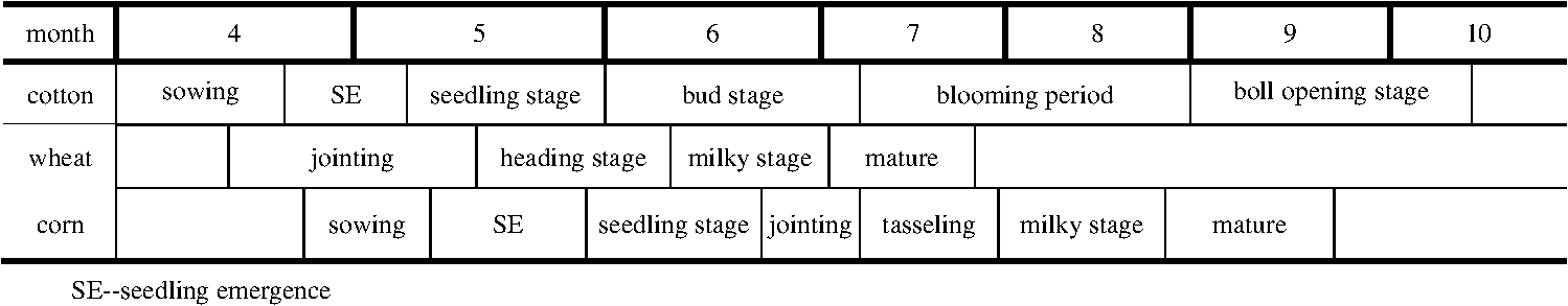
where $x$ is the threshold value of the discriminator, and $d$ is the number of the accumulated days that the pixel in the MODIS time series meets the threshold condition during the detectable period. In this study, the discriminator, $d$ , and $x$ are obtained by analyzing the MODIS time series for the detectable period discussed in Sec. 4 of this paper.

3. Study Areas and Data

3.1.

Study Areas

In order to test the threshold model methods for mapping PML, we chose southern Xinjiang, China, (Fig. 2) as our research area for three reasons. First, $> 11 %$ of PML in China is located in Xinjiang, which accounts for $> 40 %$ of the total annual cotton production in China where plastic mulch is used in 100% of the cotton fields. Second, southern Xinjiang is the key cotton plantation area in Xinjiang, accounting for $> 70 %$ of cotton acreage in the province.³² Third, the size of individual cotton fields or their aggregation in southern Xinjiang is big enough to be classified in MODIS images. To simplify the problem, we ignored the subpixel PML, which commonly occurs at the 250 m spatial resolution MODIS images, and defined PML as pixels or areas covered by $> 50 %$ plastic mulch and non-PML as $< 50 %$ covered by plastic mulch when we aggregated Landsat PML data to MODIS resolution for ground truth.

Fig. 2

The study area in southern Xinjiang, China.

The study area, which includes Shule, Shufu, and Aketao counties, is centered at 39°18’8.15”N, 76°3’33.85”E with a total of 3230 sq. km and has an arid and continental climate with a warm temperature and low annual precipitation. The average temperature is 11.3°C; the annual rainfall is $\sim 60 mm$ ;³³ and the altitude ranges between 1244 and 1353 m. Cotton, winter wheat, and spring corn are the major crop types. Cotton is usually planted between early and middle April, and winter wheat is planted before the middle October, while spring corn is planted between late April and early May (Fig. 3).

Fig. 3

Phenological calendar of major plantation in southern Xinjiang.³⁴

3.2.

Data Source and Processing

3.2.1.

MODIS time series data

MODIS has 36 bands. Among them, two have a spatial resolution of 250 m, five 500 m, and the rest have a spatial resolution of 1000 m. For PML detection, a higher spatial resolution is preferred. Therefore, the red band (620 to 670 nm, band 1) and near-infrared band (841 to 876 nm, band 2) are selected to explore temporal-spectral features for PML detection. By using the GeoBrain system developed by the Center for Spatial Information Science and System, George Mason University, USA,³⁵ MODIS surface reflectance daily L2G global 250 m Sin Grid V005 products (MOD09GQ MODIS data products) for the study area were subset and downloaded for covering the detectable period from the 85th day to the 150th day in 2009, 2013, and 2014. A batch tool, which we developed with ArcGIS ModelBuilder, was used to reproject MODIS data to the Universal Transverse Mercator coordinate system using nearest-neighbor resampling so that they can be coregistered with Landsat images used in this study.

Three time series of 250 m spatial resolution images were produced: red band (band 1), near-infrared band (band 2), and the NDVI, which is defined as the following:³⁶

NDVI = (NIR - R) / (NIR + R)

where R is the value in the red band of an image pixel and NIR is the value in the near-infrared band of an image pixel. In the study, we use MODIS band 1 as the R band and band 2 as the NIR band.

3.2.2.

Landsat images

In order to obtain the training and testing data as well as the cropland mask for this study, we manually interpreted the Landsat images for the same years as the MODIS data. Landsat images were freely downloaded from the website of Geospatial Data Cloud, China,³⁷ and the USGS official website.³⁸ Table 1 lists the images from Landsat 7 and Landsat 8 used in this study. Because of the malfunction of the Landsat 7 ETM+, image LE71490332009119SGS01 lost some scanning lines. In this study, we repaired the lost scanning lines by using the gap-fill algorithm provided by Geospatial Data Cloud website.³⁷

Table 1

Landsat level 1T data source parameters (path 149, row 33).

No.	Acquisition date and time		Entity ID	Sensor type	Average cloud cover (%)
No.	Date	GMT	Entity ID	Sensor type	Average cloud cover (%)
1	April 29, 2009	05:25	LE71490332009119SGS01	ETM+	3.51
2	May 18, 2013	05:37	LC81490332013138LGN01	OLI	2.66
3	May 05, 2014	05:34	LC81490332014125LGN00	OLI	38.28

3.3.

Ground Truths from Landsat Remote Sensing Images

One of the most economical methods for obtaining ground truths is to interpret the available relatively high-resolution satellite images (e.g., Landsat 4-5 TM, Landsat 7 ETM, or Landsat 8 OLI at 30 m spatial resolutions) since PML can be clearly visible in those images (as shown in Fig. 4). In this study, the ground truths for training and testing the TM methods were manually interpreted from the Landsat images and then aggregated to the MODIS resolution. Only part of the study area with a large concentration of PML and non-PML were interpreted. The overlay of the visually interpreted PML and non-PML from Landsat images with the MODIS time series generated the ground truths at MODIS resolution by assigning a MODIS pixel to PML if more than half of the Landsat pixels within the MODIS pixel are PML pixels. For each year, $\sim 25,000$ MODIS pixels in the study area were identified as the ground truths in this way. Among them, $\sim 10,000 pixels$ were PML pixels and the rest were non-PML pixels.

Fig. 4

Plastic-mulched landcover (PML) (purple colored) and non-PML pixels (green and gray colored) as shown on color composites of Landsat 8 OLI (RGB: bands 6, 5, 4): (a) PML (centered at 39°13’44.05”N, 76°2’11.67”E) and (b) non-PML (centered at 39°11’41.68”N, 75°57’18.70”E).

In addition to the agricultural land, the study area also contains other landuse/landcover types. Since the objective of this research is to test the effectiveness of MODIS time series data with TM methods for extraction of PML over agriculture land, a cropland mask was needed to mask out the non-agriculture land in the study area. A classification algorithm, the ML, was used to obtain the cropland mask because ML is one of the widely used classifiers with relatively high classification accuracy.³⁹ In this study, training datasets for the six landcover classes in the study area, including PML, non-PML planted land, fallow land, built-up area, water body, and bare land (such as Gobi and sand), were manually interpreted from the Landsat images and used to train the ML classifier. The trained ML classifier was used to automatically classify the Landsat images for the entire study area. The classification results were further processed with majority/minority analysis and visual correction to filter out the small spatial aggregation of classes. Table 2 shows the final classification accuracy of Landsat images. The classes of PML, non-PML planted land, and fallow land were merged into the cropland class and other three classes into the non-cropland class. Then the result was aggregated to the MODIS resolution by using the majority rule to form the cropland mask at MODIS resolution.

Table 2

Classification accuracy assessment of Landsat remote sensing images.

Time	Test data sets (pixels)		Overall accuracy (%)	Kappa coefficient	PML producer’s accuracy (%)	PML user’s accuracy (%)
Time	Cropland	Non-cropland	Overall accuracy (%)	Kappa coefficient	PML producer’s accuracy (%)	PML user’s accuracy (%)
2009	29,385	23,636	90.98	0.89	97.86	91.27
2013	28,189	20,189	89.15	0.87	95.03	87.82
2014	25,621	34,054	92.84	0.92	99.70	94.58

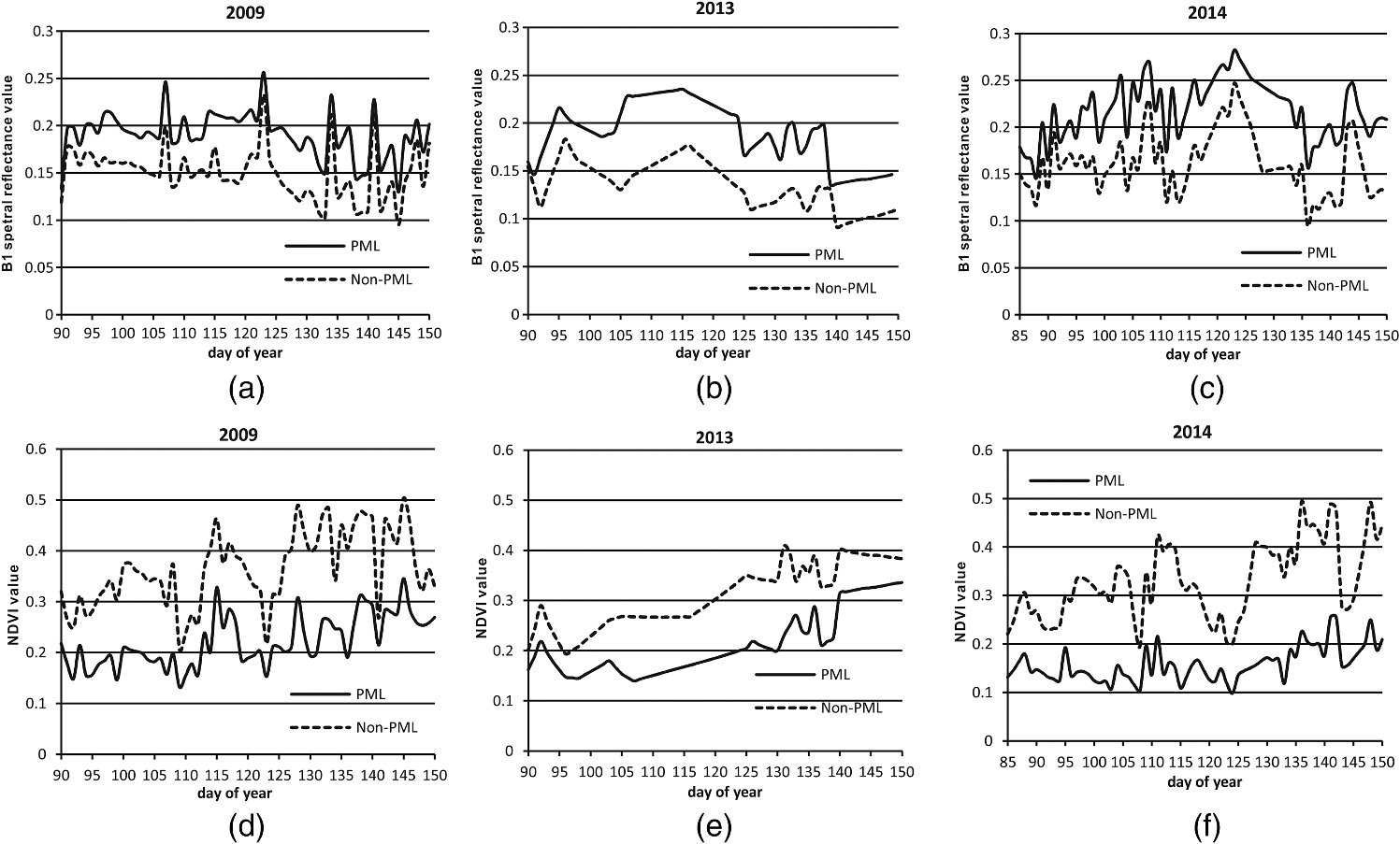
Note: PML, plastic-mulched landcover.

4. Results

4.1.

Determination of Threshold Condition and Value

There are multiple temporal-spectral features of MODIS time series useable as the discriminator for PML mapping. In order to determine the best one as the discriminator as well as its associated $d$ , and $x$ , we need to analyze the performance of different features. By using PML and non-PML training sets, we calculated the means of band 1 reflectance, band 2 reflectance, and NDVI for PML and non-PML for each day. Therefore, three pairs of daily mean spectral reflectance (DMSR) curves, which are band 1, band 2, and NDVI, are obtained from the MODIS time series for each year.

Figure 5 shows the results of the comparison of the DMSR time series between PML and non-PML using original MODIS data in 2009, 2013, and 2014. From Fig. 5, we can find that in all three years, band 1 reflectance of PML is generally higher than non-PML, while both band 2 and NDVI are just the opposite. However, there were 35 days in 2009, 43 days in 2013, and 35 days in 2014 when values of band 1, band 2, and NDVI for both PML and non-PML were very close. By checking the quality control (QC) layer of MODIS data, it was found that the dates when the values for both PML and non-PML were very close were covered by cloud either fully or partly.

Fig. 5

Comparison of daily mean spectral reflectance (DMSR) time series between PML and non-PML using the original data.

Although the study area was located in a dry region, there was frequent large cloud cover during the planting seasons. In order to remove the impact of cloud in this study, visual inspection of MODIS images was performed to find out the MODIS images with large cloud cover, which were not used in the calculation of the DMSR curve. Instead, a rebuilt image was constructed for the date of a discarded MODIS image by linearly interpolating the reflectance of individual pixels from reflectances of the corresponding pixels in good images of the nearest earlier and later good days indicted by the MODIS QC layer. For the period from the 90th to 125th day of a year, 57, 71, and 54% of MODIS images in 2009, 2013, and 2014, respectively, were discarded due to large cloud cover. After the interpolation, the means were recalculated to reconstruct the DMSR for both band 1 and the NDVI time series (Fig. 6). Band 2 time series was not reconstructed because there was no significant difference in band 2 between PML and non-PML. The reason for no significant difference is that the non-PML area in this study was mainly winter wheat, which has a high near-infrared reflectance in May. Because a large percentage of rebuilt images was used in the DMSR calculation in 2013, the curve was smoother than in other years.

Fig. 6

Comparison of DMSR time series between PML and non-PML using the interpolated data.

Figures 6(a), 6(b), and 6(c) show that, from the early sowing season to the end of the early growing season (the detectable period), the DMSR of band 1 for PML are obviously greater than that of non-PML (winter wheat and spring corn fields). The reason is that, from the time the farmers put the new transparent plastic mulch on the fields in the sowing season, the plastic mulch, which has a higher spectral reflectance in band 1, is visible in the early growing season. By further analyzing Figs. 6(a), 6(b), and 6(c), we find that the PML DMSR curves of band 1 fluctuate around 0.2, while non-PML 0.15, and this pattern of difference was the same for all the three years. Figures 6(d), 6(e), and 6(f) illustrate that the NDVI values of non-PML are above that of the PML in three years, since cotton phenology differs from that of winter wheat, namely winter wheat is in the green-up stage, while cotton is in sowing and emerging stages. Figures 6(d), 6(e), and 6(f) also show that NDVI values for non-PML in the three years of study fluctuated between 0.2 and 0.5, but generally went up with the progress of the growing season. However, the NDVI values for PML can be divided into two stages. The first stage is from the 90th day to the 125th day when the NDVI fluctuated between 0.1 and 0.25, and the second stage is from the 126th day to the 150th day when the NDVI went up with the progress of the season. Therefore, it is clear that we can use NDVI values from the 90th to 125th day (a total of 31 days), which includes the sowing and seedling emergence periods of cotton, to discriminate PML and non-PML.

To determine the best $d$ value, there were 31 training sessions with $d$ from 1 to 31. For each training session, the accuracy of PML detection was calculated by using the testing sets of ground truths. Then $d$ value with the highest detection accuracy was selected as the $d$ value of the model.

To sum up, the PML curves in NDVI of three years are all under non-PML, despite their different ranges of DMSR time series, and there is a significant difference ( $\sim 0.1$ ) between the PML and non-PML of DMSR from the 90th to the 125th day in all three years; therefore, NDVI DMSR from the 90th to the 125th day is the best discriminator to detect the PML among the three time series.

4.2.

Detecting and Mapping PML

The statement that NDVI DMSR curves for PML fluctuate around 0.2 in the three years does not mean that NDVI threshold value of detecting PML should be set to $x < 0.2$ . The reason is that DMSR values are the average spectral reflectance values of all pixels in the training sets, which means some PML pixels may have NDVI values $> 0.2$ . In other words, this threshold value will lead to the misclassification of PML pixels as non-PML pixels.

In order to avoid the misclassification, we used the threshold model to identify non-PML instead of PML in the study area and then subtracted non-PML from the croplands’ landcover images to get the PML area. According to above analysis and referring to Figs. 6(d), 6(e), and 6(f), among TM, $x$ can be 0.2. Therefore, the TM for PML detection can be written as follows:

If (the number of the accumulated days $> d$ when the NDVI value of a pixel in MODIS time series $< 0.2$ during the 95th to 125th day of a year) Then
Assign the pixel to non-PML class;
Else
Assign the pixel to PML class

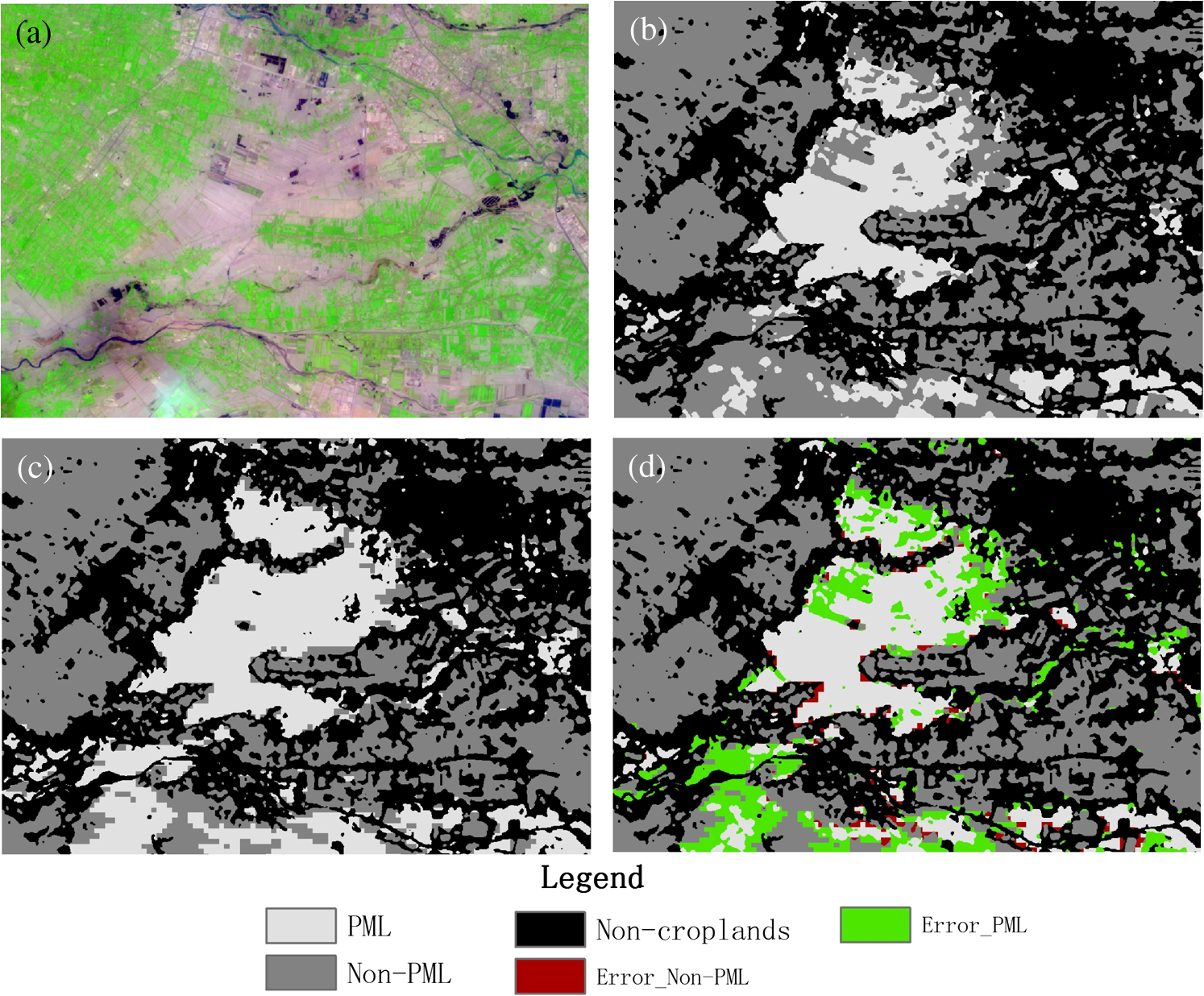
We developed a java program of TM to detect PML from MODIS NDVI time series from the 90th to the 125th day. Using PML and non-PML ground truth, the classification results were evaluated by overall accuracy (OA) and $κ$ , the kappa coefficient⁴⁰ in ENVI 5.0 software, and the results of the TM experiments are given in Table 3.

Table 3

Design and results of threshold model experiments using moderate resolution imaging spectroradiometer normalized difference vegetation index time series from 90th to 125th day.

Year	x		d
Year	x		1	2	3	4	5	6	7	8	9	10	11	12	15	16	20
2009	$< 0.2$	OA				0.760	0.836	0.841	0.848	0.848	0.843
2009		$κ$				0.431	0.643	0.651	0.660	0.656	0.643
2013		OA				0.797	0.846	0.882	0.885	0.897	*0.898*	0.896
2013		$κ$				0.587	0.689	0.763	0.773	0.796	*0.796*	0.792
2014		OA	0.819				0.753		0.838	*0.864*	0.855	0.851	0.836
2014		$κ$	0.596				0.501		0.634	*0.679*	0.658	0.655	0.633

Note: OA, overall Accuracy; italics values, the highest classification accuracy for a given year; bold values, the highest classification accuracy for a given d value and classification accuracy for the best d value.

Table 3 shows that, in 2009, when threshold parameter $x$ is 0.2 and the accumulated days parameter $d$ is 7, the classification with the TM method has achieved the highest accuracy with OA 0.848 and $κ$ 0.660, while in 2013 and 2014, when the threshold parameter $x$ is 0.2 and the accumulated days parameter $d$ is 9 and 8, respectively, classification accuracy reaches their peak with OA 0.898 and 0.864 and $κ$ 0.796 and 0.679, respectively. It also shows that we can use the same TM to detect PML with a high accuracy in three diverse years with $x = 0.2$ and $d = 8$ . OA values in all the three years are $> 0.84$ and $κ > 0.65$ . Therefore, we can conclude that TM is an effective method for mapping PML with MODIS time series data.

In order to further examine the effectiveness of the TM method, we visually compared the PML maps from MODIS with the TM method and those from Landsat with the ML classification method. To reduce the paper length, this paper only shows the MODIS and Landsat 8 OLI results for 2014 (Fig. 7). By comparing Figs. 7(a) and 7(b), we find the distribution of PML and non-PML in the two figures is very consistent.

Fig. 7

Comparison of classification results in the study area in 2014 (PML: white, non-PML: gray, non-cropland: black): (a) maximum likelihood (ML) classification map with Landsat 8 OLI and (b) threshold model classification map with moderate-resolution imaging spectroradiometer (MODIS) time serials data.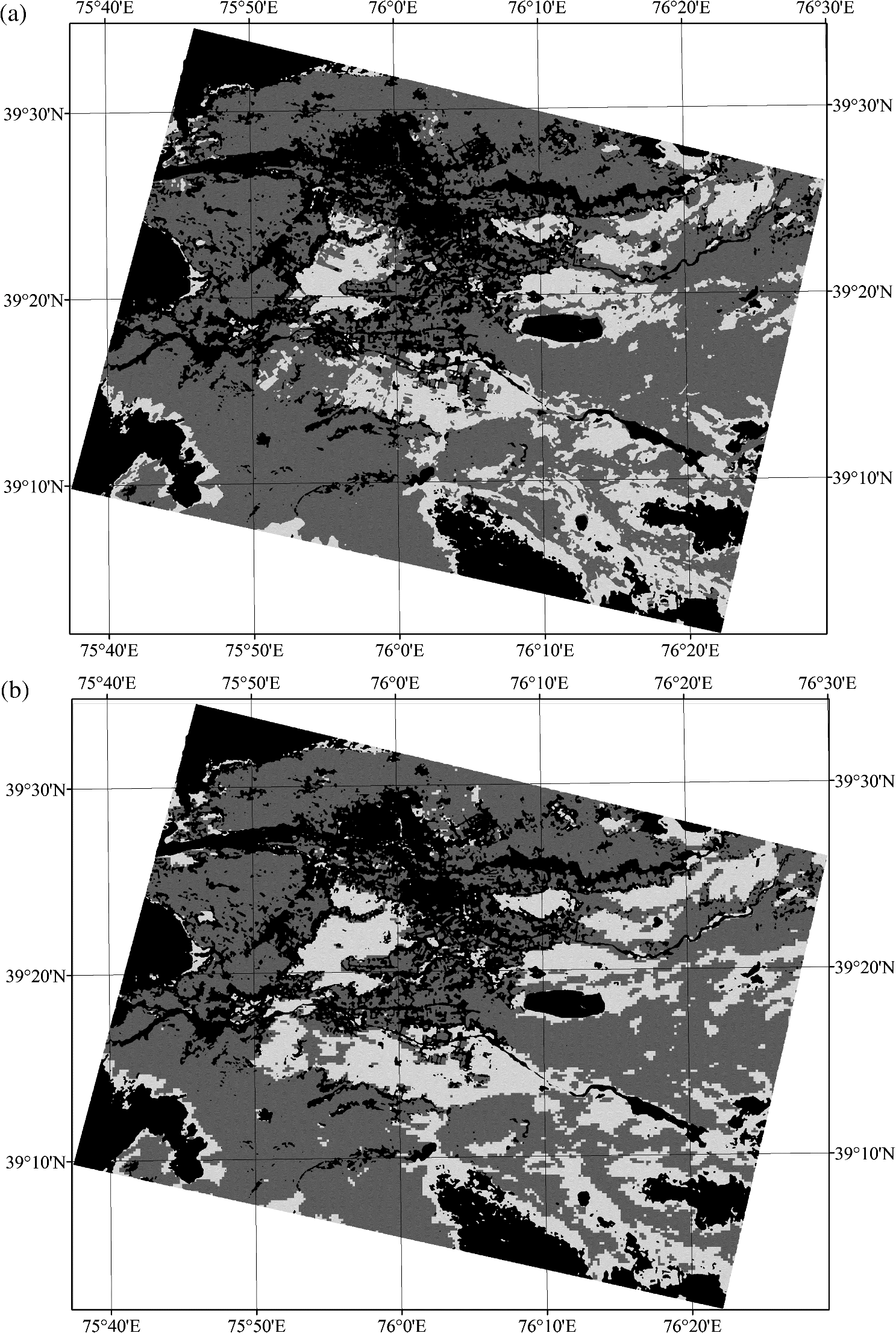

Meanwhile, we also provided Landsat 8 OLI false color composite, ML classification results with Landsat 8 OLI, and TM classification results with MODIS time serials data for part of the study area (see Fig. 8). Comparing Fig. 8(b) with Fig. 8(c), we found that the spatial distribution pattern of PML in both classification results is almost identical, but the acreages of PML resulting from MODIS is a little bit larger than that from Landsat 8 OLI. In addition, a mismatch map between Fig. 8(b) and Fig. 8(c) was created by overlaying the two PML maps with the method described in Refs. 41 and 42 and is shown in Fig. 8(d). We attribute the difference to classification errors in both the ML classifier and TM classifier.

Fig. 8

Comparison of classification results in local area in 2014: (a) Landsat 8 OLI (RGB: bands 6, 5, 4); (b) ML classification results with Landsat 8 OLI; (c) TM classification results with MODIS time serials data; (d) error of classification by comparing OLI results with MODIS results.

5. Conclusion and Discussion

From this study, we found that the interpolated NDVI DMSR time series curve in the early growing season is a good discriminator for mapping PML in Xinjiang since NDVI values of PML are all lower than that of non-PML in 2009, 2013, and 2014, respectively, and the difference between PML and non-PML curves is more significant than that in band 1 and band 2.

We designed TM experiments and successfully applied this TM to map PML from MODIS interpolated NDVI time series (from the 90th to the 125th day). Results of TM experiments show that, when the TM parameter $x$ is 0.2 and $d$ is 8, the OA and $κ$ of PML images detected by TM are $> 0.84$ and 0.65, respectively. Therefore, we believe that this accuracy can meet the needs for mapping PML over a large geographic area. Furthermore, visual comparison shows that detected locations of PML and non-PML from MODIS are consistent with the results from ML classification of Landsat images. Therefore, TM detection and mapping of PML is feasible. The PML mapping in this study is based on a croplands’ map derived from Landsat images using the ML classifier, and the accuracy of ML classifier products needs further study.

Acknowledgments

This research is supported in part by a grant from China’s National Science and Technology Support Program (Grant # 2008BAB38B05). The authors would also like to thank Ms. Qingqing Zhang, an undergraduate student from Zhejiang University, for the data preprocessing. The authors would also like to thank the reviewers for their valuable comments.

References

1.

P. Dubois, Plastics in Agriculture, 176 Applied Science Publishers, London, England (1978). Google Scholar

2.

W. J. Lamont, “What are the components of a plasticulture vegetable system?,” HortTechnology, 6 (3), 150 –154 (1996). HORTFI 1063-0198 Google Scholar

3.

M. Orzolek, “The plastic advantage,” Resource, 13 –14 (1999). Google Scholar

4.

T. Takakura and W. Fang, Climate Under Cover, 190 2nd ed.Kluwer Academic Publishers, Dordrecht (2002). Google Scholar

5.

L. Lu, L. Di and Y. Ye, “A decision-tree classifier for extracting transparent plastic-mulched landcover from Landsat-5 TM images,” IEEE J. Sel. Topics Appl. Earth Obs. Remote Sens., 7 (11), 4548 –4558 (2014). http://dx.doi.org/10.1109/JSTARS.2014.2327226 1939-1404 Google Scholar

6.

MA/PRC, China Agriculture Statistical Report 2012, (2012) , China Agriculture Press, Beijing, China ( November ). 2012). Google Scholar

7.

G. Zhou, “Analysis of situations of China agro-film industry (2010) and countermeasures for its development,” China Plast., 24 (8), 9 –12 (2010). Google Scholar

8.

P. Picuno, A. Tortora and R. L. Capobianco, “Analysis of plasticulture landscapes in Southern Italy through remote sensing and solid modelling techniques,” Landsc. Urban Plan., 100 (1–2), 45 –56 (2011). http://dx.doi.org/10.1016/j.landurbplan.2010.11.008 LUPLEZ 0169-2046 Google Scholar

9.

N. Levin et al., “Remote sensing as a tool for monitoring plasticulture in agricultural landscapes,” Int. J. Remote Sens., 28 (1), 183 –202 (2007). http://dx.doi.org/10.1080/01431160600658156 IJSEDK 0143-1161 Google Scholar

10.

F. Agüera and J. G. Liu, “Automatic greenhouse delineation from QuickBird and Ikonos satellite images,” Comput. Electron. Agric., 66 (2), 191 –200 (2009). http://dx.doi.org/10.1016/j.compag.2009.02.001 CEAGE6 0168-1699 Google Scholar

11.

E. Espí et al., “Plastic films for agricultural applications,” J. Plast. Film Sheeting, 22 (2), 85 –102 (2006). http://dx.doi.org/10.1177/8756087906064220 JPFSEH 8756-0879 Google Scholar

12.

F. Agüera, F. J. Aguilar and M. A. Aguilar, “Using texture analysis to improve per-pixel classification of very high resolution images for mapping plastic greenhouses,” ISPRS, 63 (6), 635 –646 (2008). http://dx.doi.org/10.1016/j.isprsjprs.2008.03.003 IRSEE9 0924-2716 Google Scholar

13.

E. Tarantino and B. Figorito, “Mapping rural areas with widespread plastic covered vineyards using true color aerial data,” Remote Sens., 4 (12), 1913 –1928 (2012). http://dx.doi.org/10.3390/rs4071913 17LUAF 2072-4292 Google Scholar

14.

F. Carvajal et al., “Greenhouses detection using an artificial neural network with a very high resolution satellite image,” in Proc. ISPRS Technical Commission II Symp., 37 –42 (2006). Google Scholar

15.

J. D. Colby and P. L. Keating, “Land cover classification using Landsat TM imagery in the tropical islands: the influence of anisotropic reflectance,” Int. J. Remote Sens., 19 1479 –1500 (1998). http://dx.doi.org/10.1080/014311698215306 IJSEDK 0143-1161 Google Scholar

16.

H. Thunnissen and A. D. Wit, “The national land cover database of the Netherlands,” Int. Arch. Photogramm. Remote Sens., 33 223 –230 (2000). Google Scholar

17.

F. Jacob et al., “Comparison of land surface emissivity and radiometric temperature derived from MODIS and ASTER sensors,” Remote Sens. Environ., 90 (2), 137 –152 (2004). http://dx.doi.org/10.1016/j.rse.2003.11.015 RSEEA7 0034-4257 Google Scholar

18.

J. Li, “Economic analysis of agro-film pollution in Xinjiang region,” Bord. Econ. Culture, 1 (1), 16 –17 (2008). Google Scholar

19.

Y. Li et al., “Spatio-temporal pattern dynamic of cotton plantation in Xinjiang and its driving forces,” J. Desert Res., 31 (2), 476 –484 (2011). Google Scholar

20.

J. Knorn et al., “Land cover mapping of large areas using chain classification of neighboring Landsat satellite images,” Remote Sens. Environ., 113 (5), 957 –964 (2009). http://dx.doi.org/10.1016/j.rse.2009.01.010 RSEEA7 0034-4257 Google Scholar

21.

A. B. Salberg, “Land cover classification of cloud-contaminated multitemporal high-resolution images,” IEEE Trans. Geosci. Remote Sens., 49 (1), 377 –387 (2011). http://dx.doi.org/10.1109/TGRS.2010.2052464 IGRSD2 0196-2892 Google Scholar

22.

A. R. S. Marçal et al., “Land cover update by supervised classification of segmented ASTER images,” Int. J. Remote Sens., 26 (7), 1347 –1362 (2005). http://dx.doi.org/10.1080/01431160412331291233 IJSEDK 0143-1161 Google Scholar

23.

A. Schneider, M. A. Friedl and D. Potere, “Mapping global urban areas using MODIS 500-m data: new methods and datasets based on ‘urban ecoregions’,” Remote Sens. Environ., 114 (8), 1733 –1746 (2010). http://dx.doi.org/10.1016/j.rse.2010.03.003 RSEEA7 0034-4257 Google Scholar

24.

J. Munoz-Marf, L. Bruzzone and G. Camps-Vails, “A support vector domain description approach to supervised classification of remote sensing images,” IEEE Trans. Geosci. Remote Sens., 45 (8), 2683 –2692 (2007). http://dx.doi.org/10.1109/TGRS.2007.897425 IGRSD2 0196-2892 Google Scholar

25.

J. Byeungwoo and D. A. Landgrebe, “Partially supervised classification using weighted unsupervised clustering,” IEEE Trans. Geosci. Remote Sens., 37 (2), 1073 –1079 (1999). http://dx.doi.org/10.1109/36.752225 IGRSD2 0196-2892 Google Scholar

26.

L. M. Manevitz and M. Yousef, “One-class SVMs for document classification,” J. Mach. Learn. Res., 2 139 –154 (2001). 1532-4435 Google Scholar

27.

C. Sanchez-Hernandez, D. S. Boyd and G. M. Foody, “One-class classification for mapping a specific land-cover class: SVDD classification of fenland,” IEEE Trans. Geosci. Remote Sens., 45 (4), 1061 –1073 (2007). http://dx.doi.org/10.1109/TGRS.2006.890414 IGRSD2 0196-2892 Google Scholar

28.

G. M. Foody et al., “Training set size requirements for the classification of a specific class,” Remote Sens. Environ., 104 (1), 1 –14 (2006). http://dx.doi.org/10.1016/j.rse.2006.03.004 RSEEA7 0034-4257 Google Scholar

29.

W. K. Li, Q. H. Guo and C. Elkan, “A positive and unlabeled learning algorithm for one-class classification of remote-sensing data,” IEEE Trans. Geosci. Remote Sens., 49 (2), 717 –725 (2011). http://dx.doi.org/10.1109/TGRS.2010.2058578 IGRSD2 0196-2892 Google Scholar

30.

C. B. Schaaf et al., “First operational BRDF, albedo and nadir reflectance products from MODIS,” Remote Sens. Environ., 83 (1–2), 135 –148 (2002). http://dx.doi.org/10.1016/S0034-4257(02)00091-3 RSEEA7 0034-4257 Google Scholar

31.

W. L. Stefanov and M. Netzband, “Assessment of ASTER land cover and MODIS NDVI data at multiple scales for ecological characterization of an arid urban center,” Remote Sens. Environ., 99 (1–2), 31 –43 (2005). http://dx.doi.org/10.1016/j.rse.2005.04.024 RSEEA7 0034-4257 Google Scholar

32.

G. Yang et al., “Responses of cotton growth, yield, and biomass to nitrogen split application ratio,” Eur. J. Agron., 35 (3), 164 –170 (2011). http://dx.doi.org/10.1016/j.eja.2011.06.001 EJAGET 1161-0301 Google Scholar

33.

LSSJCX/ CMA, “Kashgar precipitation figure in March 2006,” (2014) http://search.weather.com.cn/index.php?y=2006&m=03&id=51709&type1=d&type2=p&last=010000MON01&tag=HCDV_PAMS_EE0_A&td=2006/ , China Agriculture Press, Beijing, China ( December ). 2014). Google Scholar

34.

L. B. Zhao et al., “A preliminary study on the best temporal period for remote sensing to identify the cotton crops in southern and eastern Xinjiang,” China Cotton, 36 (6), 11 –14 (2008). Google Scholar

35.

L. Di, “GeoBrain—a web services based geospatial knowledge building system,” in Proc. of NASA Earth Science Technology Conf., 22 –24 (2004). Google Scholar

36.

C. J. Tucker, “Red and photographic infrared linear combinations for monitoring vegetation,” Remote Sens. Environ., 8 (2), 127 –150 (1979). http://dx.doi.org/10.1016/0034-4257(79)90013-0 RSEEA7 0034-4257 Google Scholar

37.

CNIC, “GSCloud,” (2014) http://www.gscloud.cn/ , China Agriculture Press, Beijing, China ( December ). 2014). Google Scholar

38.

USGS, “USGS earthexplorer,” (2014) http://earthexplorer.usgs.gov/ , China Agriculture Press, Beijing, China ( November ). 2014). Google Scholar

39.

J. Sun et al., “Automatic remotely sensed image classification in a grid environment based on the maximum likelihood method,” MComM, 58 (3–4), 573 –581 (2013). http://dx.doi.org/10.1016/j.mcm.2011.10.063 Google Scholar

40.

J. Cohen, “A coefficient of agreement for nominal scales,” Educ. Psychol. Meas., 20 37 –46 (1960). http://dx.doi.org/10.1177/001316446002000104 EPMEAJ 0013-1644 Google Scholar

41.

Y. Chen et al., “An evaluation of MODIS daily and 8-day composite products for floodplain and wetland inundation mapping,” Wetlands, 33 (5), 823 –835 (2013). http://dx.doi.org/10.1007/s13157-013-0439-4 0277-5212 Google Scholar

42.

C. Huang, Y. Chen and J. Wu, “Mapping spatio-temporal flood inundation dynamics at large river basin scale using time-series flow data and MODIS imagery,” Int. J. Appl. Earth Obs. Geoinf., 26 350 –362 (2014). http://dx.doi.org/10.1016/j.jag.2013.09.002 0303-2434 Google Scholar

Biography

Lulizhen Lu received the MSc and PhD degrees in cartography and geographic information systems from Zhejiang University, China, in 1996 and 2005. She is currently an associate professor with the Department of Earth Science of Zhejiang University, China. Her research interests include remote sensing image processing, feature extraction and classification, and mechanism of land use/cover change.

Danwei Hang is a graduate student pursuing her MS degree at Zhejiang University. Her research interests include mechanisms of land use/cover change and remote sensing image processing, feature extraction and classification.

Liping Di received his PhD degree in geography from the University of Nebraska-Lincoln in 1991. He is a professor and the founding director of the Center for Spatial Information Science and Systems (CSISS), George Mason University, USA. His research interests include geographic information science, geospatial information standards, geospatial cyberinfrastructure, remote sensing, global environmental changes, and large-scale geospatial information and knowledge systems.

CC BY: © The Authors. Published by SPIE under a Creative Commons Attribution 4.0 Unported License. Distribution or reproduction of this work in whole or in part requires full attribution of the original publication, including its DOI.

Citation Download Citation

Lizhen Lu, Danwei Hang, and Liping Di "Threshold model for detecting transparent plastic-mulched landcover using moderate-resolution imaging spectroradiometer time series data: a case study in southern Xinjiang, China," Journal of Applied Remote Sensing 9(1), 097094 (27 March 2015). https://doi.org/10.1117/1.JRS.9.097094

Published: 27 March 2015

Access the abstract

JOURNAL ARTICLE
14 PAGES

DOWNLOAD PAPER SAVE TO MY LIBRARY

GET CITATION

CITATIONS

Cited by 31 scholarly publications.

Explore citations on Lens.org

KEYWORDS

MODIS

Earth observing sensors

Landsat

Data modeling

Image classification

Reflectivity

Associative arrays

1.

Introduction

2.

Methodology