1.

Introduction

Over the last two decades, numerous commercial and custom-built airborne imaging systems have been developed for diverse remote sensing applications, including precision agriculture, pest management, and other agricultural applications.^1,2 Commercial availability of high resolution satellite imaging systems (e.g., GeoEye-1 and WorldView 2) in recent years provides new opportunities for remote sensing applications in agriculture.^3,4 Nevertheless, airborne imaging systems still offer some advantages over satellite imagery due to their relatively low cost, high-spatial resolution, easy deployment, and real-time/near-real-time availability of imagery for visual assessment and processing. More importantly, satellite imagery cannot always be acquired from a desired target area at specified time periods due to satellite orbits, competition for images at the same time with other customers, and weather conditions.

Unmanned aircraft systems (UAS) are being evaluated as another versatile and cost-effective platform for airborne remote sensing.^5,6 However, the safety concerns of commercial aircraft pilots, and in particular, aerial applicators and other pilots operating in low-level airspace need to be addressed before the commercial use of UAS. Today, although UAS operators can obtain an experimental airworthiness certificate for private sector (civil) UAS or a certificate of waiver or authorization (COA) for public UAS, the restrictive regulations make it very difficult to deploy UAS for practical applications in the US airspace system.

Agricultural aircraft provide a readily available and versatile platform for airborne remote sensing. Aerial applicators are highly trained pilots who use these aircraft to apply crop production and protection materials. They also protect forest and play an important role in protecting the public by controlling mosquitoes. If these aircraft are equipped with an imaging system, they can be used to acquire aerial imagery for monitoring crop growing conditions, detecting crop pests (i.e., weeds, diseases, and insect damage), and assessing the performance and efficacy of aerial application treatments. This additional imaging capability will increase the usefulness of these aircraft and help aerial applicators to generate additional revenues from remote sensing services. However, to ensure the safety of the pilot and to avoid the contamination to the camera from spray drift, the aircraft should not be used as a remote sensing platform during aerial application. Imaging equipment can be mounted onto the aircraft before or after aerial chemical application to monitor crop conditions and assess the efficacy and performance of aerial treatments.

Most of today’s airborne imaging systems are designed for use on remote sensing aircraft equipped with camera ports for research and commercial applications. These systems commonly employ multiple scientific-grade cameras equipped with different filters to obtain three or four spectral bands in the blue, green, red, and near-infrared (NIR) regions of the spectrum.^7,8 True-color images are created with the red, green, and blue bands, while color-infrared (CIR) images are produced with the NIR, red, and green bands. Some imaging systems can capture mid-infrared and far-infrared images, whereas others have the capability to take hyperspectral images from dozens to hundreds of spectral bands in the visible to thermal regions of the spectrum.

Recent advances in imaging technologies have made consumer-grade digital cameras an attractive option for remote sensing applications due to their low cost, small size, compact data storage, and ease of use. Consumer-grade digital cameras are fitted with either a charge-coupled device sensor or a complementary metal–oxide–semiconductor (CMOS) sensor. These cameras employ a Bayer color filter mosaic to obtain true-color images using one single sensor.⁹ Consequently, consumer-grade digital color cameras have been increasingly used by researchers for agricultural applications.^10–12

The Aerial Application Technology Research Unit at the US Department of Agriculture-Agricultural Research Service’s Southern Plains Agricultural Research Center in College Station, Texas, has devoted considerable efforts to the development and evaluation of airborne imaging systems as part of our research program. Currently, we have a suite of airborne multispectral and hyperspectral imaging systems for crop condition assessment, pest detection and precision aerial application.^2,8,13 Like other commercial and custom-built airborne imaging systems, these systems are either too expensive or too complex to be of practical use for aerial applicators.

To address the imaging needs of aerial applicators, low-cost, user-friendly imaging systems are needed. The objectives of this study were to: (1) assemble a low-cost, single-camera imaging system using off-the-shelf electronics; (2) develop procedures for quick image viewing and mosaicking using free and inexpensive software; and (3) demonstrate the usefulness of the imaging system for crop monitoring and pest detection.

2.

System Components and Setup

2.1.

System Components

The imaging system consisted of a Nikon D90 digital CMOS camera with a Nikon AF Nikkor 24 mm $f$/2.8D lens (Nikon Inc., Melville, New York) to capture the color image with up to $4288\times 2848$ pixels, a Nikon GP-1A GPS receiver (Nikon Inc.) to geotag the image, an AUVIO 7-in. portable LCD video monitor (Ignition L.P., Dallas, Texas) to view the live image, and a Vello FreeWave wireless remote shutter release (Gradus Group LLC, New York) to trigger the camera. The fixed focal length (24 mm) was selected to be about the same as the longer dimension of the camera sensor area ($23.6\mathrm{mm}\times 15.8\mathrm{mm}$) so that the longer dimension of the image was about the same as the flight height and the shorter dimension of the image was about 2/3 of the flight height. For example, when the image is acquired at 305 m (1000 ft) above ground level (AGL), the image will cover a ground area of approximately $305\mathrm{m}\times 201\mathrm{m}$ ($1000\mathrm{ft}\times 660\mathrm{ft}$). The major specifications of the four components are given in Fig. 1. The total cost of the four components was about $1320 with the camera and lens for $1000, the GPS receiver for $200, the monitor for $80, and the wireless trigger for $40.

Fig. 1

Major components and specifications of a low-cost imaging system.

2.3.

Camera Mounting

The camera can be attached to the bottom or the side of an aircraft with minimal or no modification to the aircraft. In our study, the camera was attached via an aluminum camera mount to the step on the right side of an Air Tractor AT-402B aircraft (Air Tractor, Inc., Olney, Texas) (Fig. 2). A similar camera mount can be built for a different aircraft.

Fig. 2

A Nikon camera mounted on the right step of an Air Tractor AT-402B. A GPS receiver and a video monitor integrated with the camera are mounted in the cockpit.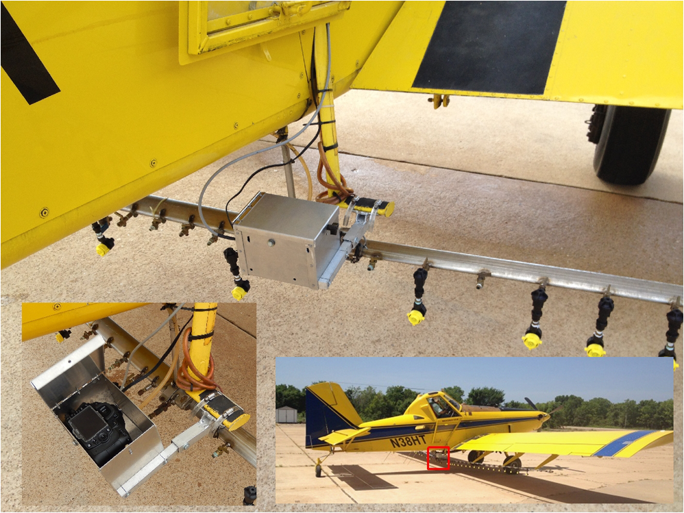

The camera was mounted such that the longer dimension of the image was perpendicular to the flight direction. To obtain nadir images, the optical axis of the camera needs to be vertical to the ground during image acquisition. The aircraft had a 7.5 deg angle from the ground with the front tilted up when parked on a flat surface. Therefore, the camera was mounted 7.5 deg tilted up in front when the aircraft was parked. When airborne, the aircraft was parallel to the ground so that nadir images were captured.

2.4.

GPS and Remote Trigger Setup

The GPS unit and the video monitor were placed in the cockpit with cable connections to the camera (Fig. 3). Since the cable provided with the GPS unit was only 25 cm (10 in) long, it was spliced and extended to 2.4 m (8 ft) long so that the GPS unit mounted near the windshield in the cockpit was able to reach the camera. The shutter release radio frequency (RF) receiver was connected to the GPS unit and the wireless RF transmitter was used to trigger the camera. It should be noted that the GPS unit only provided the coordinates for the center of the image. No gyro mount or inertia measurement unit was used in the system. Images need to be georeferenced using ground control points to create orthorectified images.

Fig. 3

Connections among four components (camera, GPS, monitor, and remote trigger) of an imaging system.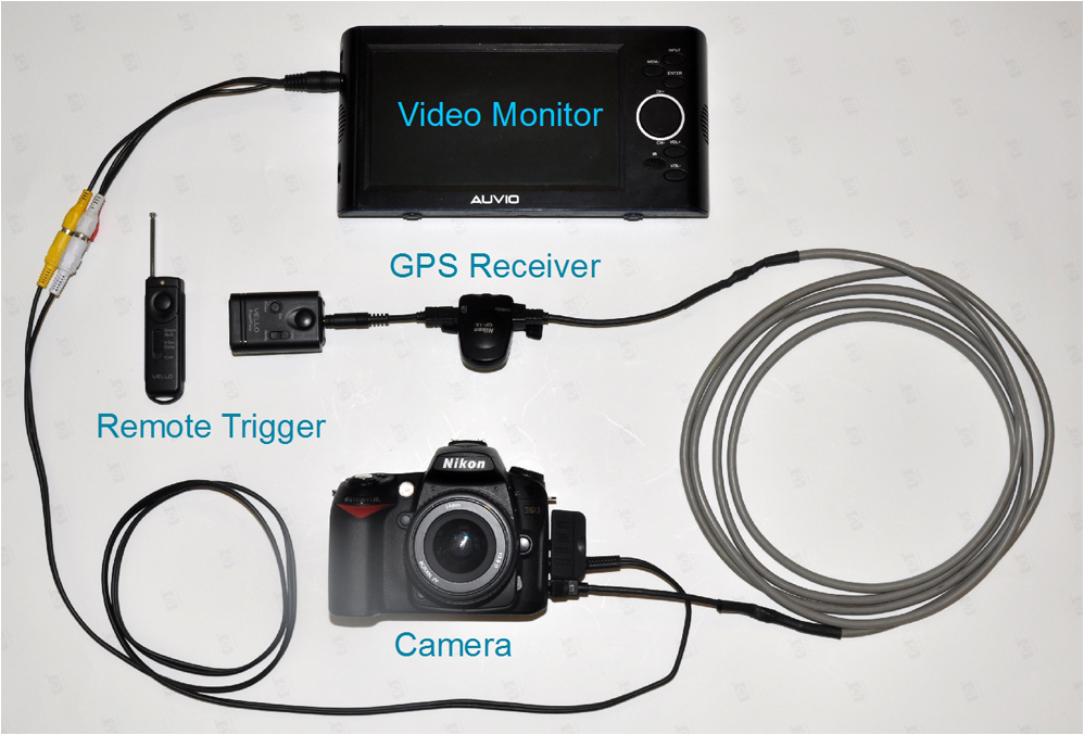

Before each image acquisition, the camera and the other components were properly set up as described above and connected as shown in Fig. 3. All batteries were fully charged, an SD memory card with sufficient storage was inserted, and a few test images were taken on the ground to make sure the whole system was working properly before takeoff.

The GP-1A GPS unit can be used with the following Nikon cameras via the GP1-CA90 cable: D90, D7000, D5100, D5000, and D3100. The prices for these cameras range from $300 to $700. The GP-1A can also be used via a different cable (GP1-CA10A) with the following more expensive Nikon cameras: D4, D3-series, D800, D800E, D700, D300-series, D2X, D2XS, D2HS, and D200. The prices range from $1700 to $8000. The setup procedures are similar for these cameras.

3.

Ground Coverage and Pixel Size Determination

The ground coverage of the camera can be determined based on the sensor size of the camera, the focal length of the lens, and the flight height of the aircraft by the following equation:

The pixel size of the fine resolution image ($4288\times 2848$ pixels) can be determined by the following equation:

Figure 1 gives the ground coverage and pixel size of the imaging system at commonly used flight heights from 152 to 3048 m (500 to 10,000 ft) AGL. When the flight height increases from 152 m (500 ft) to 3048 m (10,000 ft), pixel size increases from 3.5 cm (1.4 in.) to 70 cm (28 in.), and ground coverage increases from $\sim 150\mathrm{m}\times 100\mathrm{m}$ ($500\mathrm{ft}\times 330\mathrm{ft}$) to $3\mathrm{km}\times 2\mathrm{km}$ ($1.9\mathrm{miles}\times 1.2\mathrm{miles}$). Since flight height is normally adjusted in 500-ft or 1000-ft increments in the US, this figure can be used as a quick reference to determine appropriate flight height based on pixel size or ground coverage requirements. In practice, the width (longer dimension) of the image could be considered approximately the same as the flight height and the height (shorter dimension) of the image as 2/3 of the flight height.

4.

Image Acquisition from Individual Fields and Continuous Areas

4.1.

From Individual Fields

To take images from individual sites or fields, Google Earth 7.1 (Google Inc., Mountain View, California) was used to determine the center coordinates (latitude, longitude, and elevation) and the dimensions of the sites or fields. Based on the dimension of the imaging area, a flight height AGL was determined using Table 1. The elevation was added to the flight height to determine flight height above sea level, which is typically used on the aircraft.

Table 1

Ground coverage and pixel size of the Nikon color imaging system at different flight heights above ground level.

Flight height		Ground coverage		Pixel sizea
(m)	(ft)	(m×m)	(ft×ft)	(cm)	(in.)
152	500	$150\times 100$	$492\times 329$	3.5	1.4
305	1000	$300\times 201$	$983\times 658$	7.0	3
610	2000	$599\times 401$	$1967\times 1317$	14	6
914	3000	$899\times 602$	$2950\times 1975$	21	8
1219	4000	$1199\times 803$	$3933\times 2633$	28	11
1524	5000	$1499\times 1003$	$4917\times 3292$	35	14
1829	6000	$1798\times 1204$	$5900\times 3950$	42	17
2134	7000	$2098\times 1405$	$6883\times 4608$	49	19
2438	8000	$2398\times 1605$	$7867\times 5267$	56	22
2743	9000	$2697\times 1806$	$8850\times 5925$	63	25
3048	10000	$2997\times 2007$	$9833\times 6583$	70	28

^aPixel array set at 4288×2848 pixels.

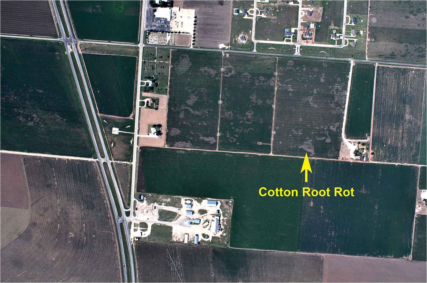
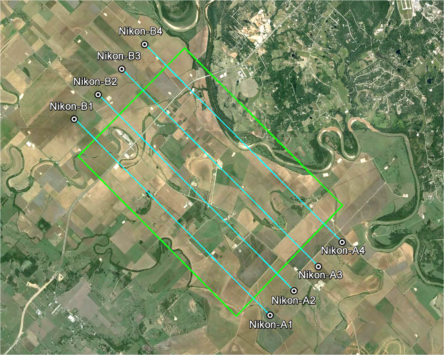
Figure 4 presents a color image taken at 1219 m (4000 ft) AGL over a corn field on July 7, 2014, near College Station, Texas. The field was located on the right side of the river and was partially damaged by feral hogs. On the color image, healthy plants have a dark green color, whereas damaged areas have a grayish tone similar to bare soil. Feral hogs, also known as wild pigs, are among the most destructive invasive species in the US today. They are both numerous and widespread throughout much of the US with an estimated population of 2.6 million in Texas alone.¹⁴ Feral hogs consume and trample crops, and their rooting and wallowing behaviors further damage crop fields.

Fig. 4

A color image acquired at 1219 m (4000 ft) AGL from a corn field with hog damage near the river near College Station, Texas.

Figure 5 shows a color image acquired at 1829 m (6000 ft) AGL over a cotton field infected with cotton root rot on October 2, 2014, near San Angelo, Texas. On the color image, healthy cotton plants have a dark green color, whereas infected plants have a grayish tone also similar to bare soil. Cotton root rot, caused by the soilborne fungus Phymatotrichopsis omnivore, is a major cotton disease affecting cotton production. Generally, only portions of the field are infected and the fungus tends to occur in similar areas over recurring years. Infected areas identified near the end of the growing season can be used for site-specific fungicide treatment in subsequent years. Airborne imagery has proven to be an accurate and effective method to map root rot infection within cotton fields.¹³

Fig. 5

A color image acquired at 1829 m (6000 ft) AGL from a cotton root rot-infected field near San Angelo, Texas.

4.2.

For Continuous and Large Areas

If a single image cannot cover the area of interest with the required pixel size, multiple images can be taken along one or more flight lines. For example, to map a $4.8\mathrm{km}\times 7.2\mathrm{km}$ ($3\mathrm{miles}\times 4.5\mathrm{miles}$) cropping area near College Station, Texas, as shown in Fig. 6, multiple images along multiple flight lines were needed. The following steps can be used to determine appropriate flight parameters:

• 1. Preset flight height, speed, and image overlap. In this example, these parameters were set at 1524 m (5000 ft) AGL, $241\mathrm{km}/\mathrm{h}$ (150 mph), and 30% in both side and forward directions, respectively.

• 2. Determine the interval between flight lines. At the flight height, each image covers $\sim 1500\mathrm{m}$ by 1000 m (5000 ft by 3300 ft). For a 30% overlap, the interval between flight lines should be $1500\mathrm{m}\times 0.7=1050\mathrm{m}$ ($5000\mathrm{ft}\times 0.7=3500\mathrm{ft}$). The distance between consecutive images should be $1000\mathrm{m}\times 0.7=700\mathrm{m}$ ($3300\mathrm{ft}\times 0.7=2310\mathrm{ft}$).

• 3. Determine the number of flight lines based on the width of the imaging area and the interval between flight lines. The width of the imaging area can be expressed as

  $$W=0.5w_0+n-1d+0.5w_0=w_0+n-1d,$$
  where $W$ is the width of the imaging area, $w_0$ is the swath of the image, $n$ is the number of flight lines, and $d$ is the interval between flight lines. Thus, the number of flight lines, $n$, can be calculated by

  Eq. (4)

  $$n=1+\frac{W-w_0}{d}.$$

  In this example, $W=4.8\mathrm{km}=4800\mathrm{m}$ ($3\text{miles}=15840\mathrm{ft}$), $w_0=1500\mathrm{m}$ (5000 ft) and $d=1050\mathrm{m}$ (3500 ft), so $n=1+(4800-1500\mathrm{m})/1050$ $\mathrm{m}=4.1$ or $n=1+(\mathrm{15,840}-5000\mathrm{ft})/3500$ $\mathrm{ft}=4.1$. If some extra area was already considered in the predetermined imaging area, four flight lines should be enough; otherwise, five flight lines should be used to cover the required imaging area.

• 4. Determine the imaging rate (framing frequency) along the flight lines. For a 30% overlap, the distance between consecutive images should be 700 m (2310 ft) as determined in step 2). At $241\mathrm{km}/\mathrm{h}$ (150 mph) or $241\times 1000/3600=67\mathrm{m}/\mathrm{s}$ ($150\times 5280/3600=220\mathrm{ft}/\mathrm{s}$), the time it takes to fly such a distance is $700/67=10.4\mathrm{s}$ ($2310/220=10.5\mathrm{s}$). Thus, the imaging rate should be approximately one image for every 10 s.

Fig. 6

A $4.8\mathrm{km}\times 7.2\mathrm{km}$ ($3\text{miles}\times 4.5\text{miles}$) cropping area (green box) near College Station, Texas.

In this example, to take continuous images over a $4.8\mathrm{km}\times 7.2\mathrm{km}$ ($3\mathrm{miles}\times 4.5\mathrm{miles}$) cropping area at 1500 m (5000 ft) AGL with a ground speed of $241\mathrm{km}/\mathrm{h}$ (150 mph) and to achieve a 30% image overlap along and between the flight lines, images were acquired at 10-s intervals along four flight lines spaced at 1050-m (3500-ft) intervals. The coordinates of the two end points of each flight line were determined from the lower left corner of the imaging area (the green box in Fig. 6) using Google Earth. First, a distance equal to half of the image swath (750 m or 2500 ft) was measured from the lower left corner of the green box toward the lower right corner as the beginning point for the first flight line. Then, a distance equal to the interval between the flight lines (1050 m or 3500 ft) was measured out to determine the beginning points for the rest of the flight lines. The same procedure was repeated at the upper left corner of the imaging area to determine the ending points for all the flight lines. To provide the pilot with enough time and distance to align the aircraft along the flight lines, the beginning and ending points were extended to outside of the image area by $\sim 900\mathrm{m}$ (3000 ft), as shown in Fig. 6. Finally, the latitude and longitude coordinates for all the points were recorded and provided to the pilot for navigation during image acquisition.

5.

Image Viewing and Mosaicking

Both the NEF and JPEG images stored in the SD card can be readily viewed with the ViewNX software (Nikon Inc.) supplied with the camera, though the JPEG images can be viewed with any image viewer installed on a computer such as Windows Photo Viewer. The supplied ViewNX software can also be used to export the NEF image as Tiff and other format for further processing.

To quickly view the images and their geographic locations, Google’s image viewer Picasa 3.9 (Google Inc.) was used to create a KMZ file from geotagged images. The free software can be downloaded at Ref. 15. To view all the images, use “File→Add Files to Picasa” to load all the geotagged images. To create a KMZ file, select all the geotagged JPG or NEF images and then use “Tools→Geotage→Export” to “Google Earth File.”

Figure 7 shows the geotagged images (thumbnails) for the above example in Google Earth using the KMZ file created in Picasa. From the plot, the user can quickly identify individual images for particular fields and study sites, or a group of continuous images that can be mosaicked together to cover a larger geographic area for quick assessment of crop conditions.

Fig. 7

Geotagged images plotted in Google Earth. The images were acquired at 1524 m (5000 ft) above ground level near College Station, Texas.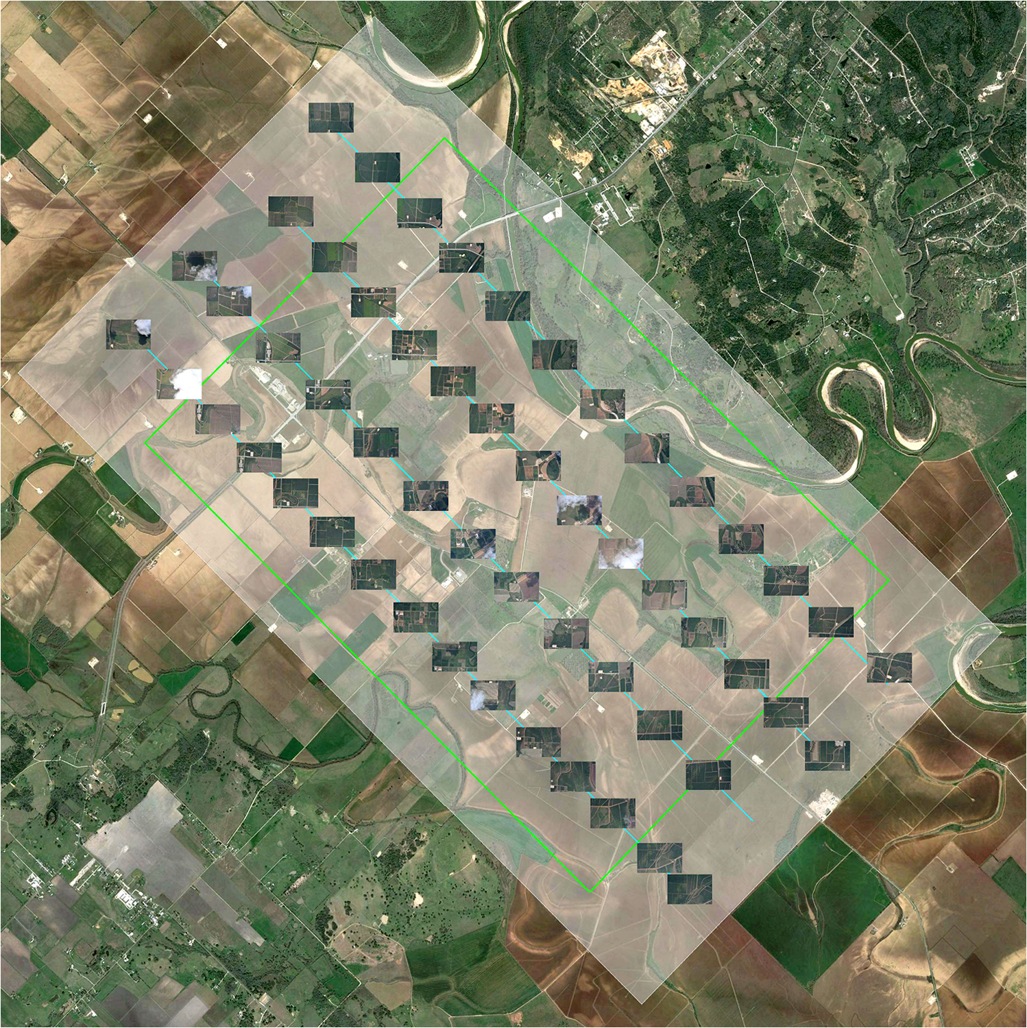

Image mosaicking is the process of combining multiple photographic images with overlapping fields of view to produce a panorama or mosaicked high resolution image. Many computer software programs can mosaic multiple images and a popular example is Adobe Photoshop, which includes a tool known as Photomerge. Adobe Photoshop CC (Adobe Systems Incorporated, San Jose, California) is recommended for image mosaicking since it not only performs seamless mosaicking for a large number of images simultaneously but also gives you a complete set of useful tools for image processing and analysis. The cost of the subscription-based software was $19.99 per month with an annual plan.

Figure 8 presents a mosaicked image from all 42 geotagged images within the green box as shown in Fig. 7 using Adobe Photoshop CC. The software did an excellent job of mosaicking the individual images together as one seamless image. The individual images seem to be positioned accurately and seamlessly to provide a continuous coverage of the cropping area. A few clouds and shadows near the center of the imaging area can be seen on the mosaicked image. The quality of the mosaic depends to a large extent on the quality of the individual images; therefore, to minimize the distortion and discontinuity in the mosaicked image, it is important that nadir images be taken with sufficient overlap under sunny and relatively calm conditions.

Fig. 8

A mosaicked image from all 42 images within the green box shown in Fig. 8 using Adobe Photoshop CC.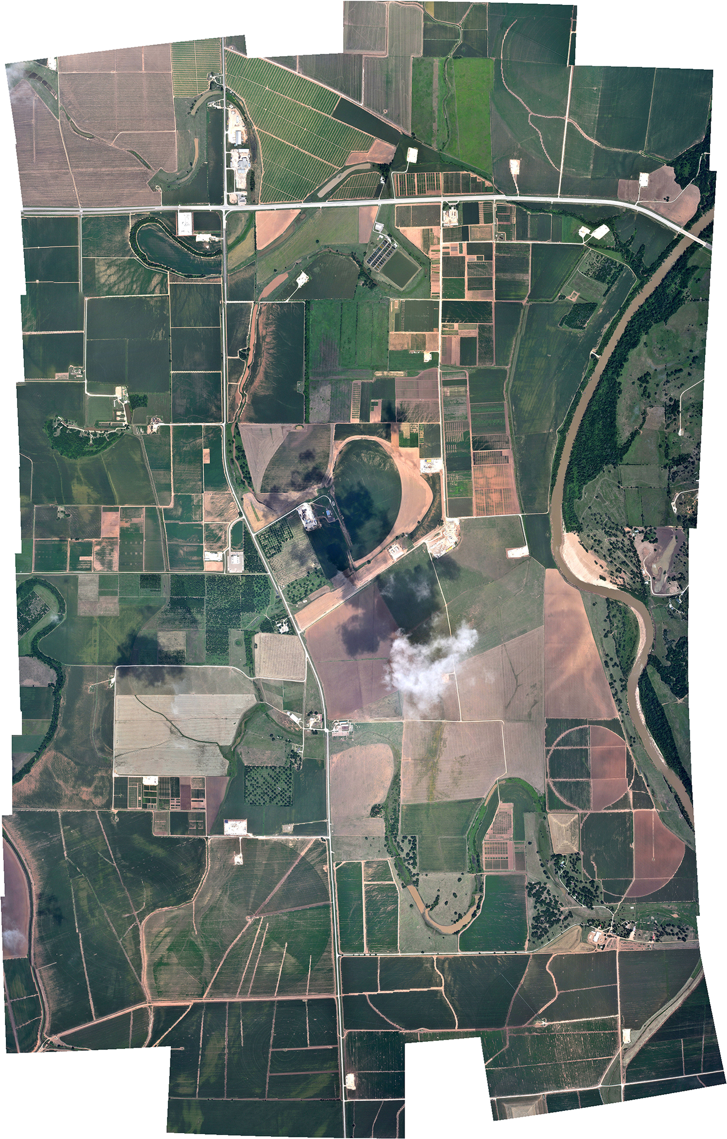

Based on our experience, it took 1 to 2 h to create and enter the flight lines into a navigation system, half an hour to setup and check the imaging system, another half an hour to acquire the images, and less than an hour to download the images, view them on a PC and then mosaic them together. Therefore, if an aerial applicator or a user is familiar with the imaging system and the software (i.e., Google Earth, Picasa and Adobe Photoshop CC) used for flight planning and image mosaicking, it should take 3 to 4 h to complete the imaging mission for such a geographic area.

It should be noted that geotagged images taken with the imaging system only contain the center coordinates of the images, but they are not georeferenced. Mosaicking modules in professional image processing software generally require that the images to be mosaicked be georeferenced. However, Adobe Photoshop CC does not need the images to be georeferenced for image mosaicking. Although not georeferenced, these individual images and mosaicked images can be readily used to visually assess crop conditions and identify problem areas within fields and over large geographic areas. Thus, real-time or near-real-time management decisions can be made to address the problems. Nevertheless, the mosaicked image should not be used for quantitative image analysis because of potential positional error. Images need to be georeferenced and classified to generate prescription maps for site-specific treatment or management. Although expensive and sophisticated image processing software is commercially available, free or inexpensive and user-friendly software is needed for image georeferencing and classification for aerial applicators.

6.

Image Analysis for Two Example Applications

To illustrate the usefulness and accuracy of the low-cost imaging system for crop condition assessment and pest detection, this section presents the analysis of the two sample images shown in Figs. 4 and 5 for mapping feral hog-damaged areas in the corn field and cotton root rot-infected areas in the cotton field. Conventional image processing methods and professional software were used for the analysis.

The images were georeferenced or rectified to the Universal Transverse Mercator, World Geodetic Survey 1984 (WGS-84), Zone 14, coordinate system based on a set of ground control points around the fields located with a Trimble GPS Pathfinder ProXRT receiver (Trimble Navigation Limited, Sunnyvale, California). The root mean square errors for rectifying the images were within 1 m. The images were resampled to 1-m resolution using the nearest neighborhood technique. All procedures for image rectification and classification were performed using ERDAS Imagine software (Intergraph Corporation, Madison, Alabama).

The color images were classified into 2 to 12 spectral classes using ISODATA unsupervised classification.¹⁶ A five-class classification map for the corn field and a six-class classification map for the cotton field provided the best separability among the classes. The spectral classes in each classification map were then grouped into affected and nonaffected zones by comparison with the original image and based on ground observations. The merged two-zone classification maps for the two fields were then used to estimate the hog-damaged and root rot-infected areas, respectively.

For accuracy assessment of the two merged two-zone classification maps, 60 random points for the corn field and 100 points for the cotton field were selected and ground-checked using the Trimble GPS receiver. An error matrix for each two-zone classification map was generated by comparing the classified classes with the actual classes based on ground verification. Classification accuracy measures, including overall accuracy, kappa coefficient, producer’s accuracy and user’s accuracy, were calculated based on each of the two error matrices.¹⁷

6.1.

Hog Damage Assessment

Figure 9 shows the five-class classification map (b) and the merged two-zone map (c) for the corn field with hog damage. A visual comparison of the classification maps and the original color image (a) indicated that the five-class classification map effectively identified apparent hog-damaged areas and other crop growth variability within the field. The pink and red colors correspond to hog-damaged areas, whereas blue, green, and dark green colors depict the nondamaged areas. Classification results showed that 1.2 ha (3.0 ac) or 15.6% of the 7.8-ha (19.3-ac) corn field was damaged by feral hogs.

Fig. 9

(a) Color image, (b) five-class unsupervised classification map, and (c) merged two-zone map for a corn field with hog damage in San Angelo, Texas.

Table 2 summarizes the accuracy assessment results for the hog-damaged corn field. The overall accuracy of the classification map was 91.7%, indicating that the probability of image pixels being correctly identified in the classification map is 91.7%. The producer’s accuracy (a measure of omission error), which indicates the probability of actual areas being correctly classified, was 91.3% for the hog-damaged category and 91.9% for the nondamaged category. In other words, 91.3% of the hog-damaged areas were correctly identified as damaged (or 8.7% of the damaged areas were incorrectly identified as nondamaged) in the classification map. This omission error was partly due to the small inclusions of damaged plants within nondamaged areas. The user’s accuracy (a measure of commission error), which is indicative of the probability that a category classified on the map actually represents that category on the ground, was 87.5% for the hog-damaged and 94.4% for the nondamaged areas. Another accuracy measure, the kappa estimate for this field, was 0.825, indicating that the classification achieved an accuracy that is 82.5% better than would be expected from random assignment of pixels to categories.

Table 2

Accuracy assessment results for a two-zone classification map of a normal color image for corn field with hog damage.

Classified category	Actual category		Total	User’s accuracy
	Damaged	Nondamaged
Damaged	21	3	24	87.5%
Nondamaged	2	34	36	94.4%
Total	23	37	60
Producer’s accuracy	91.3%	91.9%

Note: Overall accuracy=(21+34)/60=91.7%. Kappa=0.825

6.2.

Cotton Root Rot Detection

Figure 10 shows the six-class unsupervised classification map (b) and the merged two-zone map (c) for the cotton field infected with cotton root rot. A visual comparison of the classification maps and the original color image (a) indicated that the six-class classification map effectively identified apparent root rot areas and other crop growth variability within the field. The magenta and red colors correspond to root rot areas, whereas blue, cyan, green, and dark green colors show the noninfected areas. Classification results showed that 3.3 ha (8.2 ac) or 12.2% of the 27.4-ha (67.6-ac) cotton field was infected by root rot.

Fig. 10

(a) Color image, (b) six-class unsupervised classification map and (c) merged two-zone map for a cotton field infected with cotton root rot in San Angelo, Texas.

Table 3 shows the accuracy assessment results for the root rot-infected cotton field. The overall accuracy of the classification map was 93%, indicating that 93% of the image pixels were correctly identified in the classification map. The producer’s accuracy was 92.3% for the root rot category and 93.8% for the noninfected category. The user’s accuracy was 94.1% for the root rot areas and 91.8% for the noninfected areas. The kappa estimate for this field was 0.860.

Table 3

Accuracy assessment results for a two-zone classification map of a normal color image for a cotton field infected with cotton root rot.

Classified category	Actual category		Total	User’s accuracy
	Infected	Noninfected
Infected	48	3	51	94.1%
Noninfected	4	45	49	91.8%
Total	52	48	100
Producer’s accuracy	92.3%	93.8%

Note: Overall accuracy=(48+45)/100=93.0%. Kappa=0.860

7.

Summary and Discussion

A low-cost, user-friendly airborne imaging system was assembled using off-the-shelf electronics in this study. The system, consisting of a consumer-grade color camera, a GPS receiver, a video monitor, and a remote trigger, can be easily installed to any agricultural aircraft for airborne remote sensing. Normal color images with $4288\times 2848$ pixels can be captured and stored in 12-bit raw (NEF) and 8-bit JPEG format at altitudes of 152 to 3050 m (500 to 10,000 ft) to achieve pixel sizes of 3.5 to 70 cm (1.4 to 28 in.). A set of optimal parameters of the camera was identified to allow images to be acquired under various altitudes, speeds, and ground cover conditions.

Operational procedures were developed for system setup, flight planning, image acquisition, image viewing, and image mosaicking, and a user’s manual was written to provide step-by-step guidance for aerial applicators and end users. Geotagged images taken from individual sites or a large geographic area can be viewed and mosaicked together using free and inexpensive software. Our experience indicated that it took less than 4 h for an experienced user to produce a mosaicked image covering a $36\text{-}{\mathrm{km}}^2$ ($14{\text{miles}}^2$) area from the time to plan the imaging mission. However, more research is needed to determine the positional accuracy for content-based mosaicked images based on known ground control points and compare the positional accuracy between the content-based mosaicking method and other mosaicking methods.

Extensive airborne testing of the imaging system has shown that the system is very reliable and user friendly and requires minimum maintenance. The images from the system are high quality and can be opened in any image processing software. Accuracy assessment of images taken from a hog-damaged corn field and a root rot-infected cotton field has demonstrated that color images alone can be useful for crop monitoring and pest detection. Sample images collected from other study sites have also shown that the imaging system can be used for mapping crop weeds and other remote sensing applications.

The total cost of the system was under US$1500, including camera mount construction and GPS cable splicing. An aerial applicator or any end user can easily assemble such a system with the off-the-shelf electronics using the methods and techniques presented in this study. If a Nikon D90 or another Nikon camera is selected, the other system components can be the same. Otherwise, a compatible GPS unit is needed for the selected camera. Similar procedures can be used to determine optimal camera parameters and flight coverage information. With the addition of a low-cost, user-friendly imaging system to an agricultural aircraft, the aerial applicator will be able to monitor crop conditions in the areas to be sprayed and identify potential obstacles and sensitive areas to be avoided during aerial application. This additional information can increase the efficiency and safety of aerial application operations. Meanwhile, the additional imaging capability will allow the aerial applicator to generate additional revenues from remote sensing services.

Although all types of remote sensing platforms and imaging systems are available, various factors have to be considered as to which is more appropriate for a particular application, including the size of the area to be mapped, complexity of the associated plant communities, and time and cost constraints. UAS have a great potential as a cost-effective remote sensing platform. Currently, there are still many restrictions on their use for commercial applications. High resolution satellite systems can cover large areas with relatively fine spatial resolution. Satellite imagery can be cost-effective for large geographic areas, but it may not be available when it is needed for time-sensitive applications. Therefore, manned aircraft provide an alternative between UAS and satellite platforms. As far as the imaging systems are concerned, single RGB cameras are inexpensive and easy to use but may not be sufficient for some applications for early pest detection or differentiation of similar plant species, for which more sophisticated multispectral and hyperspectral imagery may be needed.

The use of images with visible and NIR bands is very common in remote sensing, especially for vegetation monitoring. Many vegetation indices such as the normalized difference vegetation index require spectral information in the NIR and red bands. Consumer-grade cameras only provide the three broad visible bands. If NIR band images are needed, filtering techniques can be used to convert a color camera to a NIR camera. With a second camera to collect NIR images, it will be necessary to align the color and NIR images from the two cameras. Although it is common to use multiple cameras and the alignment procedure is routinely done by remote sensing specialists, it will be a challenge for aerial applicators to perform these tasks without a lot of training and experience.

To obtain NIR and red bands from a single standard RGB camera, the NIR blocking filter in the camera can be removed and then a long-wave pass filter is added to remove blue wavelengths. NIR and red bands are computed as specific linear combinations of the three resulting channels.¹⁸ This approach has been used by Tetracam Inc. (Chatsworth, California) in its single camera-based ADC series imaging systems that can capture CIR images with NIR, red, and green bands. However, the smoothing effect involved in the process reduces image spatial resolution and the linear combinations to create the NIR and red bands amplify image noise.¹⁸ Therefore, the single RGB camera-based imaging system will serve as a good first step to add imaging capability to agricultural aircraft.

As aerial applicators become more familiar with the simple imaging system, additional capability can be added. Color images alone can be useful for agricultural applications as demonstrated by the two example applications. We are in the process of identifying and/or developing user-friendly software that can be used to perform basic image processing and create prescription maps for precision application without the use of expensive and sophisticated commercial image processing software. Meanwhile, we will continue evaluating the single-camera system and compare it with other more sophisticated multispectral and hyperspectral imaging systems for monitoring crop conditions, detecting crop pests, and assessing aerial applications. Continued testing and research will help us to better understand the capability and limitations of the low-cost imaging system and allow us to enhance and expand its capability to meet aerial applicators’ remote sensing needs.