Backscattering modeling of wheat using vector radiative transfer theory

Bo Huang; Yan Chen; Lei He; Ling Tong; Yong Wang

doi:10.1117/1.JRS.9.097093

21 April 2015 Backscattering modeling of wheat using vector radiative transfer theory

Bo Huang, Yan Chen, Lei He, Ling Tong, Yong Wang

Author Affiliations +

Journal of Applied Remote Sensing, Vol. 9, Issue 1, 097093 (April 2015). https://doi.org/10.1117/1.JRS.9.097093

Abstract

A microwave backscattering model of winter wheat based on the vector radiative transfer theory has been established. The model focused on the distribution of wheat ears that are directly related to the yield. In addition, characteristics of the wheat growth have been adequately considered. Compared to the measured values, the model effectively simulated the microwave backscattering characteristics of winter wheat. Intercomparison of the winter wheat model and modified Michigan Microwave Canopy Scattering (MIMICS) model using experimental data shows that the winter wheat model had better cross-polarized simulation results than the modified MIMICS model did. This improvement was attributed to the special attention paid to the cross-polarization after the booting stage. After booting, wheat ear started to appear and grow in size. Wheat ear contributed greatly to cross-polarized backscatter. The inclusion of the ear as one of the model components was significant in modeling the observed cross-polarized backscattering.

1. Introduction

Wheat productivity is related to food security, which plays an important role in social stability and economic development. Thus, the monitoring of growth and output in wheat areas is critical. Due to the pervasive cloud presence in some locations where wheat is planted, continuous monitoring using optical remote sensing is impossible. With the advantage of acquiring data at all-weather conditions, microwave remote sensing is helpful. Moreover, with the development of the microwave backscattering model, one can not only model the backscatter under different growing stages, but also invert the model to estimate the wheat yield.

It is well known that the backscattering coefficient is not only affected by the radar system parameters such as frequency, polarization, and incident angles, but also the surface parameters such as soil roughness and moisture, and presence and structure of vegetation. In order to monitor the surface vegetation, researchers have applied many different theories such as the vector radiative transfer (VRT) theory, analytic wave theory of random media, and the discrete scatter theory to understand the scattering mechanism from vegetated surface or wheat field in this case.

The Michigan Microwave Canopy Scattering (MIMICS) model based on the VRT theory has been developed to simulate the radar backscattering from a forested environment for the forest.¹ The model is successful and is widely used.²^–⁵ Toure et al.⁶ modified the MIMICS model for the wheat at the L- and C-bands in 1994. Their model explained horizontal–horizontal polarization (HH) backscattering mechanisms well at the L- and C-bands. A coherent polarimetric microwave scattering model for grassland was developed.⁷^,⁸ Marliani et al.⁹ used the coherent electromagnetic model to compute the backscattering coefficient of wheat and sunflowers during the growing season, which demonstrates the potential of the interferometric observation on the crop classification algorithms based on scattering mechanisms. Champion et al.¹⁰ built the semiempirical model to simulate the backscattering coefficient of a wheat crop and confirmed that the radar configuration had a similar role to the canopy structure in the control of the radar backscattering coefficient. Cookmartin et al.¹¹ and Brown et al.¹² presented a comprehensive multilayer second-order radiative transfer model, which showed that the second-order terms contributed no more than 0.5 dB to the backscattering coefficient at all polarizations from wheat. Picard et al.¹³^–¹⁶ also presented a second-order backscatter model for wheat canopies based on numerical solution of the multiple scattering Foldy–Lax equation and omitted the leaves and ears. Del Frate et al.¹⁷ developed an algorithm based on the radiative transfer theory to monitor the soil moisture and growth cycle of wheat.

The above models focused on the microwave backscattering characters of wheat in various aspects using a scatter mechanism and experimental data, and promoted the development of the microwave scattering theory. To a certain degree, their models simulated the components as ideal scatters and had to omit the influence of other components, thus complex formation of backscatter presents a tough task for modeling research. Closely examining the above models, one observes some deficiency in the modeling of backscattering especially the underestimation of the cross-polarized term. One possible cause is the exclusion of wheat ears in the modeling. Therefore, a microwave backscattering model of winter wheat-based on the VRT theory is presented. A wheat ear is one of the scattering components in modeling. Descriptions of the model development and verification as well as model prediction of wheat yield are detailed.

2. Model

In modeling, winter wheat is divided into two types of scattering components (wheat stem and wheat leaves) before the heading period. After the heading, model component for wheat ears is added as the third component (Fig. 1). The soil under the wheat crop is assumed to be a random rough surface. The stem is modeled as a vertical finite length cylinder and the leaf is modeled as an ellipsoid with a limited leaf inclination angle. The wheat stem and leaf are distributed evenly in the vertical range from $z = - d$ to $z = 0$ before the heading period. The wheat ears modeled as elliptical scatterers within a layer between $z = 0$ and $z = - h$ are inserted ( $d$ : aggregate thickness; $h$ : ears thickness) (Fig. 1). M0 could be taken as the soil contribution; M1 represents the individual contribution from wheat leaves, while M2 indicates stems; M3 indicates wheat ears’ response, and M4 can be explained as mixed contributions from wheat parameters and other corresponding parameters. As demonstrated in the previous studies as well as this study, the one-layer scattering model is suitable to simulate the backscatter from wheat, especially before the heading stage. The addition of the second layer to the model should accommodate for the scattering contribution from wheat ears after the heading. The new vertical variable for the extinction matrix and phase matrix should account for full polarimetric scattering of the nonuniform distributed and elliptical scatter,¹⁸ which is the cause for the improvement in the simulation of cross-polarized backscattering.

Fig. 1

The scattering mechanisms from wheat (a) before the heading stage and (b) after the heading stage.

The VRT is given in Eq. (1):¹⁸

Eq. (1)

\frac{d I (r, \hat{s})}{d s} = - {\bar{k}}_{e} (\hat{s}) \cdot I (r, \hat{s}) + \int d s^{'} \bar{P} (s, s^{'}) \cdot I (r, s^{'}) .

The VRT equation describes the scattering, absorbed, multiple scattering, and transferred processes of electromagnetic wave intensities [Stokes intensities $I (r, \hat{S})$ ] along the direction. The extinction matrix ${\bar{k}}_{e}$ describes the attenuation of $I (r, \hat{S})$ caused by scatter and absorption. The phase matrix describes the multiple scattering progresses from direction $(θ^{'}, ϕ^{'})$ to direction $(θ, ϕ)$ .

By means of the forward-scattering theorem, the extinction matrix can be written as¹⁸

Eq. (2)

{\bar{k}}_{e} (θ, φ) = \frac{4 π}{k} n_{0} Im [\hat{p} \cdot \bar{S} (θ, ϕ; θ, ϕ) \cdot \hat{p}] = \frac{2 π}{k} n_{0} [\begin{matrix} 2 Im 〈 S_{v v}^{0} 〉 & 0 & Im 〈 S_{v h}^{0} 〉 & - Re 〈 S_{v h}^{0} 〉 \\ 0 & 2 Im 〈 S_{h h}^{0} 〉 & Im 〈 S_{h v}^{0} 〉 & Re 〈 S_{h v}^{0} 〉 \\ 2 Im 〈 S_{h v}^{0} 〉 & 2 Im 〈 S_{v h}^{0} 〉 & Im 〈 S_{v v}^{0} + S_{h h}^{0} 〉 & Re 〈 S_{v v}^{0} - S_{h h}^{0} 〉 \\ 2 Re 〈 S_{h v}^{0} 〉 & - 2 Re 〈 S_{v h}^{0} 〉 & Re 〈 S_{h h}^{0} - S_{v v}^{0} 〉 & Im 〈 S_{v v}^{0} + S_{h h}^{0} 〉 \end{matrix}],

where

S_{p q}^{0}

(

p, q = v, h

) is an element of the forward-scattering matrix

{\bar{S}}^{0} = \bar{S} (θ, ϕ; θ, ϕ)

. The extinction matrix can be expressed as a figure for spherical particles, and a diagonal matrix for the nonspherical particles is uniformly distributed in the horizontal direction.

The phase matrix is a transfer matrix which describes the scattering energy transfer from direction $(θ^{'}, ϕ^{'})$ to direction $(θ, ϕ)$ , which has a similar definition as that of the Mueller matrix. The matrix is given by¹⁸

Eq. (3)

\bar{P} (θ, ϕ; θ^{'}, ϕ^{'}) = n_{0} [\begin{matrix} 〈 {| S_{v v} |}^{2} 〉 & 〈 {| S_{v h} |}^{2} 〉 & Re 〈 S_{v v} S_{v h}^{*} 〉 & - Im 〈 S_{v v} S_{v h}^{*} 〉 \\ 〈 {| S_{h v} |}^{2} 〉 & 〈 {| S_{h h} |}^{2} 〉 & Re 〈 S_{h v} S_{h h}^{*} 〉 & - Im 〈 S_{h v} S_{h h}^{*} 〉 \\ 2 Re 〈 S_{v v} S_{h v}^{*} 〉 & 2 Re 〈 S_{v h} S_{h h}^{*} 〉 & Re 〈 S_{v h} S_{h h}^{*} + S_{v h} S_{h v}^{*} 〉 & - Im 〈 S_{v v} S_{h h}^{*} - S_{v h} S_{h v}^{*} 〉 \\ 2 Im 〈 S_{v v} S_{h v}^{*} 〉 & 2 Im 〈 S_{v h} S_{h h}^{*} 〉 & Im 〈 S_{v v} S_{h h}^{*} + S_{v h} S_{h v}^{*} 〉 & Re 〈 S_{v v} S_{h h}^{*} - S_{v h} S_{h v}^{*} 〉 \end{matrix}] .

According to the VRT theory, the extinction matrix mentioned in Eq. (4) is given by Eq. (2). Thus, we can get the VRT equations of this model¹⁸^,¹⁹

Eq. (4)

θ \frac{d}{d z} I_{r}^{+} (θ, ϕ, z) = - K_{r}^{+} (θ, ϕ) \cdot I_{r}^{+} (θ, ϕ, z) + F_{r}^{+} (θ, ϕ, z),

Eq. (5)

- θ \frac{d}{d z} I_{r}^{-} (- θ, ϕ, z) = - K_{r}^{-} (- θ, ϕ) \cdot I_{r}^{-} (- θ, ϕ, z) + F_{r}^{-} (- θ, ϕ, z) .

In Eqs. (4) and (5), $I_{r}^{+} (θ, ϕ, z)$ and $I_{r}^{-} (- θ, ϕ, z)$ are the upward and downward Stokes intensities, $K_{r}^{\pm}$ is the extinction matrix, and $F_{r}^{+} (θ, ϕ, z)$ and $F_{r}^{-} (- θ, ϕ, z)$ are the scattering source functions which represent the scattering contribution by the wheat layer. The phase matrix mentioned in Eq. (6) is given by Eq. (3).

These scattering source functions are²⁰^,²¹

Eq. (6)

F_{r}^{+} (θ, ϕ, z) = \frac{1}{θ} [\int_{0}^{2 π} \int_{0}^{1} P_{r} (θ, ϕ; θ^{'}, ϕ^{'}) I_{r}^{+} (θ^{'}, ϕ^{'}, z) d θ^{'} d ϕ^{'} + \int_{0}^{2 π} \int_{0}^{1} P_{r} (θ, ϕ; - θ^{'}, ϕ^{'}) I_{r}^{-} (- θ^{'}, ϕ^{'}, z) d θ^{'} d ϕ^{'}],

Eq. (7)

F_{r}^{-} (- θ, ϕ, z) = \frac{1}{θ} [\int_{0}^{2 π} \int_{0}^{1} P_{r} (- θ, ϕ; θ^{'}, ϕ^{'}) I_{r}^{+} (θ^{'}, ϕ^{'}, z) d θ^{'} d ϕ^{'} + \int_{0}^{2 π} \int_{0}^{1} P_{r} (- θ, ϕ; - θ^{'}, ϕ^{'}) I_{r}^{-} (- θ^{'}, ϕ^{'}, z) d θ^{'} d ϕ^{'}],

where

P_{r} (θ, ϕ; θ^{'}, ϕ^{'})

is the phase matrix and describes the scattering property from direction

(θ^{'}, ϕ^{'})

into direction

(θ, ϕ)

.

In order to solve Eqs. (4) and (5), one needs to have the boundary conditions given as²⁰^,²¹

Eq. (8)

I_{r}^{-} (- θ, ϕ, z = 0) = I_{0} δ (θ - θ_{0}) \cdot δ (ϕ - ϕ_{0}),

Eq. (9)

I_{r}^{+} (- θ, ϕ, z = - h) = R_{w} (θ) \cdot I_{r}^{-} (- θ, ϕ, z = - h),

where

I_{0}

is the incident Stokes intensity,

δ

is an impact function, and

0 \leq θ \leq π / 2

.

R_{w}

is the Mueller matrix of the ground surface.

Solving Eqs. (4)–(9) iteratively as a group, one can obtain the first-order solution²⁰

Eq. (10)

I^{b s} (θ_{0}, ϕ_{0}) = I_{1}^{+} (θ_{0}, ϕ_{0} \pm π, z = 0) = T (θ_{0}, ϕ_{0}) I_{0},

with

Eq. (11)

T (θ_{0}, ϕ_{0}) = \frac{1}{θ_{0}} Q D_{r} (θ_{0}, ϕ_{0} \pm π; - h / θ_{0}) \cdot Q^{- 1} R_{w} (θ_{0}, ϕ_{0} \pm π) Q A_{1} Q^{- 1} \cdot R_{w} (θ_{0}, ϕ_{0}) D_{r} (θ_{0}, ϕ_{0}; - h / θ_{0}) Q^{- 1} + \frac{1}{θ_{0}} Q D_{r} (θ_{0}, ϕ_{0} \pm π; - h / θ_{0}) \cdot Q^{- 1} R_{w} (θ_{0}, ϕ_{0} \pm π) Q A_{2} Q^{- 1} + \frac{1}{θ_{0}} Q A_{3} Q^{- 1} R_{w} (θ_{0}, ϕ_{0}) \cdot Q D_{r} (θ_{0}, ϕ_{0}; - h / θ_{0}) \cdot Q^{- 1} + \frac{1}{θ_{0}} Q A_{4} Q^{- 1} + Q A_{5} Q^{- 1},

where

Q

is a matrix formed by the eigenvectors of the extinction matrix and

Q^{- 1}

is the inverse matrix of

Q

.

D_{r}

is a diagonal matrix related to the eigen values of

K_{r}

. It is given by

Eq. (12)

D_{r} {(θ, ϕ; - z / θ)}_{(i, i)} = \exp [- λ_{i} (θ, ϕ) z / θ],

where

λ_{i}

is the

i

’th eigen value of

K_{r}

.

$A_{1}$ to $A_{5}$ (Ref. 20) in Eq. (11) are given as

Eq. (13)

A_{1} = \int_{- h}^{0} D_{r} (- θ, ϕ; - (z^{'} + h) / θ) Q^{- 1} P_{r} (- θ, ϕ; θ_{0}, ϕ_{0}) Q D_{r} (θ_{0}, ϕ_{0}; - (z^{'} + h) / θ_{0}) d z^{'}

Eq. (14)

A_{2} = \int_{- h}^{0} D_{r} (- θ, ϕ; - (z^{'} + h) / θ) Q^{- 1} P_{r} (- θ, ϕ; θ_{0}, ϕ_{0}) Q D_{r} (- θ_{0}, ϕ_{0}; z^{'} / θ_{0}) d z^{'}

Eq. (15)

A_{3} = \int_{- h}^{0} D_{r} (θ, ϕ; z^{'} / θ) Q^{- 1} P_{r} (θ, ϕ; θ_{0}, ϕ_{0}) Q D_{r} (θ_{0}, ϕ_{0}; - (z^{'} + h) θ_{0}) d z^{'}

Eq. (16)

A_{4} = \int_{- h}^{0} D_{r} (θ, ϕ; z^{'} / θ) Q^{- 1} P_{r} (θ, ϕ; - θ_{0}, ϕ_{0}) Q D_{r} (- θ_{0}, ϕ_{0}; z^{'} / θ_{0}) d z^{'}

Eq. (17)

A_{5} = D_{r} (θ, ϕ; - h / θ) Q^{- 1} R_{w} (θ, ϕ; - θ_{0}, ϕ_{0}) Q D_{r} (- θ_{0}, ϕ_{0}; - h / θ_{0}) .

Therefore, the backscattering coefficient of wheat is

Eq. (18)

σ_{VV}^{0} = 4 π θ_{0} {[T]}_{11,} σ_{VH}^{0} = 4 π θ_{0} {[T]}_{12,} σ_{HV}^{0} = 4 π θ_{0} {[T]}_{21,} σ_{HH}^{0} = 4 π θ_{0} {[T]}_{22} .

3. Experiments

The study area is at the crop research and demonstration site of Qianjin Town, Qionglai County, Sichuan Province, China. The location is 30°24′22.29″N and 103°32′15.97″E. The topography is gentle with an elevation at 487 m above mean sea level. The site is jointly managed and owned by the University of Electronic Science and Technology of China and Sichuan Agriculture University. Winter wheat is one of the research and demonstration crops, and its growth period is about 200 days from November to May. The studied wheat area is 3 ha.

A scatterometer (Table 1) was used to collect the backscattering coefficient during the period of wheat growth. Measurements at 11 time intervals (Table 2) were completed. At each time interval, full polarized C-band data were collected with elevation angles ranging from 10 deg to 70 deg with an increment of 3 deg. The C-band is chosen because its wavelength is similar to that of the wheat and it is sensitive to wheat parameters such as leaves. The measured backscattering coefficients’ value is the average of 6 to 9 measurements (in 6 to 9 different measurements, the azimuths are different at the same incident angle). It should be noted that the booting and filling stages are the most critical growth phases to determine the wheat productivity. The booting stage is the final stage of vegetative growth, which lays a solid foundation for the reproductive growth if the growth is flourishing [Fig. 2(a)]. In the filling stage [Fig. 2(b)], the wheat stores starch, protein, and other organic materials produced by photosynthesis in the grain, which is the crucial moment for the harvest.

Table 1

System parameters of C-band ground-based scatterometer.

Center frequency	5.3 GHz
Polarization	HH/VV/VH/HV
Bandwidth	$\geq 0.6 GH$
Work system	frequency-modulated continuous-wave
Operation slant range	$\geq 100 m$
Transmit power	$\geq 50 mw$
Dynamic range	$\geq 45 dB$
Measurement accuracy	0.5 dB
Range of elevation angle	0 deg to 90 deg
Range of azimuth angle	0 deg to 359 deg
Receiving antenna beam width	6 deg
Transmitting antenna width	8 deg

Table 2

Measurement schedule at 11 time intervals.

Growth phase	Date	Growing days since seeding
Infantile state	13 Nov 2010	15
Two leaves	3 Dec 2010	35
The early stage of tillering	25 Dec 2010	57
The late stage of tillering	14 Jan 2011	77
Jointing stage	25 Feb 2011	119
Flag leaf stage	4 Mar 2011	126
Booting stage	19 Mar 2011	141
Heading stage	1 Apr 2011	153
Flowering stage	16 Apr 2011	168
Filling stage	29 Apr 2011	181
Mature stage	18 May 2011	200

Fig. 2

The photos of wheat (a) during the booting stage and (b) during the filling stage.

After the processing of the initial field data, values at the booting and filling stages were obtained as shown in Table 3. All data were mean values. The stalk moisture and ear moisture were derived from the fresh weight and dry weight of the stalk and ears, respectively. The correlation length and roughness of the ground surface were obtained by digitizing the surface (vertical) profile photographed against white boards at the sample site.

Table 3

The parameter list of the wheat and ground surface data at the booting and filling stages.

Model parameters	At booting stage	At filling stage
Leaf thickness (m)	0.0002	0.00026
Leaf minor axis (m)	0.0175	0.0168
Leaf major axis (m)	0.229	0.206
Leaf moisture (%)	88.3	62.3
Leaf density ( $/ m^{3}$ )	1490	1392
Stalk length (m)	0.455	0.67
Stalk radius (m)	0.0028	0.0026
Stalk moisture (%)	89.7	74.2
Stalk density ( $/ m^{3}$ )	298	348
Height of wheat crops (m)	0.621	0.86
Ear length (m)		0.14
Ear radius (m)		0.0052
Ear moisture (%)		63.1
Ear density ( $/ m^{3}$ )		2137
Surface correlation length (m)	0.08072	0.08072
Surface roughness (m)	0.00636	0.00636
Soil moisture (%)	27.4	22.9

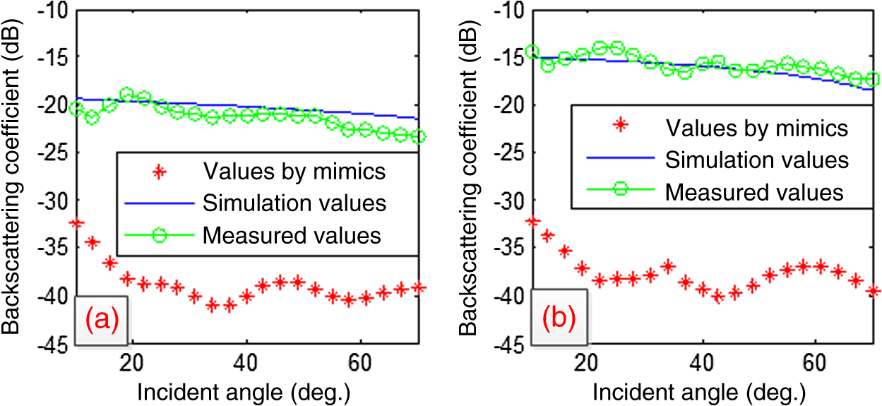
The parameterization of the structural parameters of wheat for extinction and phase matrices was on the basis of Jin and Xu.²⁰

4. Results and Discussions

Even though scatterometer and field measurements were conducted at 11 time intervals, modeling at the booting and filling stages was given next because of the stated importance in wheat productivity. The growth and output situations are highly related to the booting stage and filling stage. Therefore, the simulation results in these two stages are compared with the measured values and simulation results of the modified MIMICS model. When putting MIMICS into the wheat scattering characteristic research, the common methods simplify its tall tree structure. We take the wheat stem as the main branch, wheat leaves as tree leaves, ears as secondary branches. The trunk has to be omitted since it has a large body.

4.1.

Comparison Between Simulation Values Modeled with Measured Values

Observed and measured C-band HH, vertical–vertical polarization (VV), and horizontal–vertical polarization (HV) backscatter coefficients versus incidence angles at the booting and filling stages were shown in Fig. 3. Figures 3(a), 3(c), and 3(e) were at the booting stage, and Figs. 3(b), 3(d), and 3(f) were at the filling stage. Results in HH-, VV-, and HV-polarizations were the first, second, and third rows, respectively. Figure 3(a) is the HH-polarization, while the second row is the VV-polarization, and the third row is the VH-polarization. As shown in Fig. 3, both the observed and simulated backscatter coefficients vary with the change of incidence angles. At each incidence angle and each polarization, there might be a general agreement between the observed and modeled values since the maximum difference was less than 3 dB overall (Fig. 3). Multipolarized simulation results and measured values at the C-band vary with incidence angles. Because the HV-polarization curve is similar to that of the VH-polarization, it has not been shown here. The maximum difference between the measured values and simulation results is no more than 3 dB. Thus, it can be concluded that the simulation results from the wheat microwave backscattering model agree well with the values measured in a real-world situation. In this experiment, numerous variables affect the measurement accuracy, thus the range of 3 dB error could be taken as the normal error in the microwave scattering measurement. Around the previously mentioned two stages, since backscatter is sensitive to the flag leaves, the flag leaves might cause the oscillation of backscattering with the variation of incidence angles. The backscattering coefficients decreased and produced the wave valley in these curves. The previous researchers show that the backscattering coefficient decreases with an increase in the incidence angles. Otherwise, the curve was different from the actual situation, the reason of which could be the simplification of the extinction matrix and phase matrix. Figure 3 shows the simulation and the measured values. The main reason for this fit that is the measured data selected from the measured data base can fits the simulation well. Meanwhile, the measured data had quite a bit of difference compared to the simulation results from modified MIMICS. We consider it suitable to compare the measured data to the simulation results by our model.

Fig. 3

Comparison of simulation and measured values at the booting stage (a, c, and e) and filling stage (b, d, and f). First row—HH, second row—VV, and third row—HV. (a) Booting stage, HH-polarization, (b) filling stage, HH-polarization, (c) booting stage, VV-polarization, (d) filling stage, VV-polarization, (e) booting stage, VH-polarization, and (f) filling stage, VH-polarization.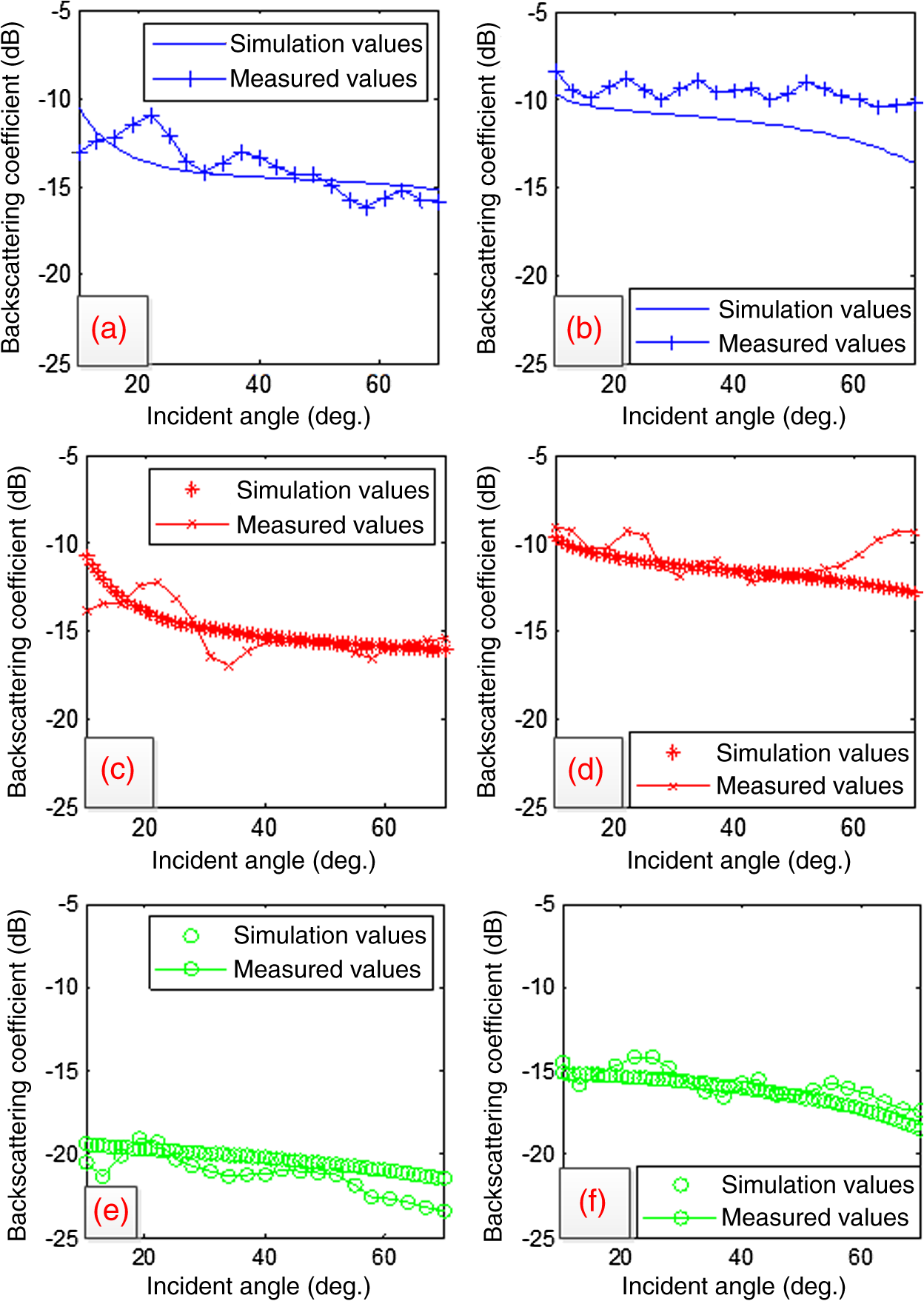

4.2.

Backscattering Coefficients Comparison among Values by Model, Values from MIMICS and Values Measured by Scatterometer

The MIMICS model was developed for radar backscattering in a forested environment. The usefulness of this model for vegetation such as wheat was explored. When the model is applied to wheat, there is no obvious stratification between the stalk and canopy. The tree trunk does not exist. In this study, a wheat stem was treated as a main branch in MIMICS model, a wheat leaf as a “tree” leaf, and a wheat ear as a secondary branch. The tree trunk is ignored. With these modifications, modeled results were obtained. As compared to the observed values, there was an overall agreement in the copolarized backscatter coefficients. However, modeled HV backscattering coefficients were significantly lower than those observed (Fig. 4). A possible cause was attributed to the cross-polarized backscattering simulated in modified MIMICS and underestimated in the modification. The simulation value of the model built in the paper is flat because the simplification of the extinction matrix and phase matrix make the model less effectiveness than the modified MIMICS model. The cross-polarized backscattering is primarily derived from multiscattering phenomena. However, when the MIMICS model is applied to simulate the wheat scattering value, several M4 values contributing to cross-polarized backscattering are omitted. The removal of trunks leads to no second-order scattering item for the trunk–ground interactions. The second-order term is another important contributor to the cross-polarized backscattering. Second, the secondary branch and the leaf have the same ranges in MIMICS, but the ears and the leaves of wheat have different ranges. If the wheat ear is taken as the secondary branch, errors result.

Fig. 4

Cross-polarized backscattering values versus incidence angles (a) at the booting stage and (b) at the filling stage.

4.3.

HV Backscattering Coefficients After Booting Stage

After the booting stage or 141 days since seeding in this study, the model component for the wheat ear was added to the model. The assessment was carried out with the incidence angles ranging from 20 deg to 70 deg. The component contributed greatly to cross-polarized backscatter, whereas the component of the copolarized scattering could be limited. The cross-polarized backscatter was elevated by the inclusion of this component (Fig. 5). At an incident angle of 30 deg, the elevated value increased as the growing season continued after booting. The different values between the simulation values without ears and those actually measured reached a maximum at 200 growth days, the mature stage in the wheat growth cycle.

Fig. 5

The measured values and the simulation values of cross-polarized versus growing days (sim-value infers to simulation values).

4.4.

Discussion

The model proposed in this paper simulated the backscatter at two stages, the booting and filling stages, respectively. Focusing on the booting stage, the research studied the microwave characteristics of wheat and prepared a comparison of the backscattering values between wheat with and without ears. Because protein, starch, and organic matter are assimilated in the grain by photosynthesis in the filling stage, the research chose the filling stage as the study stage. The research aim is to propose a model that can better simulate the backscattering coefficients for wheat with ears. The stages with and without ears could be compared in the model. We could find the result without ears had quite a difference from the measured ones, while the results with ears agreed well with the measured results (Fig. 5), so the simulation results of the model showed the ears play a key role in the backscatter contribution after booting stage, and could verify the assumption we proposed the exclusion of wheat ears in modeling could cause the underestimation of cross polarization. Taking wheat ears as a necessary modeling component is acceptable. However, the model has some disadvantages compared with the modified MIMICS model. The copolarization simulation results were not applicable and had worse effects than the modified MIMICS model of wheat. The model should be modified to fit the full-polarization data and promoted to fit normal situations such as moisture and roughness of soil, topography, and wheat parameters. The next step for developing the model is adding the microwave characteristics of wheat with ears to the yields’ impact factors (soil moisture, temperature, soil moisture, variety and growth parameters wheat, and so on) and build the wheat yields’ estimation model.

5. Conclusion

A backscattering model for wheat has been developed using the VRT theory. The layer of wheat crop is comprised of two kinds of scattering particles before the heading period, the wheat stem and the leaf of wheat, and three kinds of scattering particles after the heading period, the wheat stem, the wheat leaf, and the wheat ear. To account for the influence on wheat ear, two submodels were designed. Before the booting stage, there was no wheat ear. The first submodel consisted of wheat stem and leaf layer over ground surface. After booting, the model component for the wheat ear was added. Thus, the second submodel included the stem, leaf, and ear over the ground surface.

Compared to the measured values, the accuracy of the proposed model prove that the proposed model has a better cross-polarization than MIMICS by comparing the simulation results of the proposed model to the measured values and simulation results of the MIMICS model.

On the basis of this model, the paper analyzed the cross-polarized backscattering coefficients and found that the wheat ears have considerable impact on the cross-polarization. The results may be used to interpret remote sensing images, monitor the crop growth, and make predictions of the crop production.

Acknowledgments

This work is supported by the National Natural Science Foundation of China (Nos. 41371340 and 41071222). The Prior Research Program of the 12th Five-year Civil Aerospace Plan (D040201-04).

References

1.

F. T. Ulaby et al., “Michigan microwave canopy scattering model,” Int. J. Remote Sens., 11 (7), 1223 –1253 (1990). http://dx.doi.org/10.1080/01431169008955090 IJSEDK 0143-1161 Google Scholar

2.

P. Liang et al., “Radiative transfer model for microwave bistatic scattering from forest canopies,” IEEE Trans. Geosci. Remote Sens., 43 (11), 2470 –2484 (2005). http://dx.doi.org/10.1109/TGRS.2005.853926 IGRSD2 0196-2892 Google Scholar

3.

P. Liang et al., “Radar backscattering model for multilayer mixed-species forests,” IEEE Trans. Geosci. Remote Sens., 43 (11), 2612 –2627 (2005). http://dx.doi.org/10.1109/TGRS.2005.847909 IGRSD2 0196-2892 Google Scholar

4.

A. Monsivais-Huertero et al., “Microwave electromagnetic modelling of Sahelian grassland,” Int. J. Remote Sens., 31 (7), 1915 –1943 (2010). http://dx.doi.org/10.1080/01431160902926582 IJSEDK 0143-1161 Google Scholar

5.

M. Brolly and I. H. Woodhouse, “Long wavelength SAR backscatter modeling trends as a consequence of the emergent properties of tree populations,” Remote Sens., 6 (8), 7081 –7110 (2014). http://dx.doi.org/10.3390/rs6087081 2072-4292 Google Scholar

6.

A. Toure et al., “Adaptation of the MIMICS backscattering model to the agricultural context-wheat and canola at L and C bands,” IEEE Trans. Geosci. Remote Sens., 32 (1), 47 –61 (1994). http://dx.doi.org/10.1109/36.285188 IGRSD2 0196-2892 Google Scholar

7.

J. M. Stiles and K. Sarabandi, “Electromagnetic scattering from grassland. I. A fully phase-coherent scattering model,” IEEE Trans. Geosci. Remote Sens., 38 (1), 339 –348 (2000). http://dx.doi.org/10.1109/36.823929 IGRSD2 0196-2892 Google Scholar

8.

J. M. Stiles, K. Sarabandi and F. T. Ulaby, “Electromagnetic scattering from grassland. II. Measurement and modeling results,” IEEE Trans. Geosci. Remote Sens., 38 (1), 349 –356 (2000). http://dx.doi.org/10.1109/36.823930 IGRSD2 0196-2892 Google Scholar

9.

F. Marliani et al., “Simulating coherent backscattering from crops during the growing cycle,” IEEE Trans. Geosci. Remote Sens., 40 (1), 162 –177 (2002). http://dx.doi.org/10.1109/36.981358 IGRSD2 0196-2892 Google Scholar

10.

I. Champion, L. Prevot and G. Guyot, “Generalized semi-empirical modelling of wheat radar response,” Int. J. Remote Sens., 21 (9), 1945 –1951 (2000). http://dx.doi.org/10.1080/014311600209869 IJSEDK 0143-1161 Google Scholar

11.

G. Cookmartin et al., “Modeling microwave interactions with crops and comparison with ERS-2 SAR observations,” IEEE Trans. Geosci. Remote Sens., 38 (2), 658 –670 (2000). http://dx.doi.org/10.1109/36.841996 IGRSD2 0196-2892 Google Scholar

12.

S. Brown et al., “Wheat scattering mechanisms observed in near-field radar imagery compared with results from a radiative transfer model,” in Proc. IEEE 2000 Int. Geoscience and Remote Sensing Symp. (IGARSS 2000), 2933 –2935 (2000). Google Scholar

13.

G. Picard et al., “A second order backscatter model for wheat canopies. Formulation and comparison with data,” in Proc. IEEE 2001 Int. Geoscience and Remote Sensing Symp. (IGARSS’01), 1368 –1370 (2001). Google Scholar

14.

G. Picard et al., “A backscatter model for wheat canopies. Comparison with C-band multiparameter scatterometer measurements,” in Retrieval of Bio-and Geo-Physical Parameters from SAR Data for Land Applications, 291 –296 (2002). Google Scholar

15.

G. Picard and T. Toan, “A multiple scattering model for C-band backscatter of wheat canopies,” J. Electromagn. Waves Appl., 16 (10), 1447 –1466 (2002). http://dx.doi.org/10.1163/156939302X00093 JEWAE5 0920-5071 Google Scholar

16.

G. Picard, T. Le Toan and F. Mattia, “Understanding C-band radar backscatter from wheat canopy using a multiple-scattering coherent model,” IEEE Trans. Geosci. Remote Sens., 41 (7), 1583 –1591 (2003). http://dx.doi.org/10.1109/TGRS.2003.813353 IGRSD2 0196-2892 Google Scholar

17.

F. Del Frateet al., “Wheat cycle monitoring using radar data and a neural network trained by a model,” IEEE Trans. Geosci. Remote Sens., 42 (1), 35 –44 (2004). http://dx.doi.org/10.1109/TGRS.2003.817200 IGRSD2 0196-2892 Google Scholar

18.

Y. Jin and F. Xu, The Vector Radiative Transfer Theory and Parameter Inversion, 1st ed.Science Press, Henan (1994). Google Scholar

19.

F. Xu and Y. Jin, “Numerical simulation of fully polarimetic scattering from a layer of hybrid non-spherical particles above a randomly rough surface,” J. Microwaves, 21 (6), 1 –7 (2005). 1005-6122 Google Scholar

20.

Y. Jin and F. Xu, Theory and Approach for Polarimetric Scattering and Information Retrieval of SAR Remote Sensing, 1st ed.Science Press, Beijing (2008). Google Scholar

21.

Y. Jin, Remote Sensing Theory of Electromagnetic Scattering and Thermal Emission, 1st ed.Science Press, Beijing (1993). Google Scholar

Biography

Bo Huang is studying in the School of Automation Engineering at the University of Electronic Science and Technology of China. His research fields include microwave measurement and modeling, and crop growth monitoring.

Yan Chen is a professor in the School of Automation Engineering at the University of Electronic Science and Technology of China. Her research fields include theory of microwave remote sensing, scattering mechanism and image processing.

Biographies of the other authors are not available.

CC BY: © The Authors. Published by SPIE under a Creative Commons Attribution 4.0 Unported License. Distribution or reproduction of this work in whole or in part requires full attribution of the original publication, including its DOI.

Citation Download Citation

Bo Huang, Yan Chen, Lei He, Ling Tong, and Yong Wang "Backscattering modeling of wheat using vector radiative transfer theory," Journal of Applied Remote Sensing 9(1), 097093 (21 April 2015). https://doi.org/10.1117/1.JRS.9.097093

Published: 21 April 2015

Access the abstract

JOURNAL ARTICLE
11 PAGES

DOWNLOAD PAPER SAVE TO MY LIBRARY

GET CITATION

CITATIONS

Cited by 6 scholarly publications.

Explore citations on Lens.org

KEYWORDS

Backscatter

Ear

Scattering

Data modeling

Microwave radiation

Radiative transfer

Polarization

1.

Introduction

2.

Model

Fig. 1

Eq. (1)

Eq. (2)

Eq. (3)

Eq. (4)

Eq. (5)

Eq. (6)

Eq. (7)

Eq. (8)

Eq. (9)

Eq. (10)

Eq. (11)

Eq. (12)

Eq. (13)

Eq. (14)

Eq. (15)

Eq. (16)

Eq. (17)

Eq. (18)

3.

Experiments

Table 1

Table 2

Fig. 2

Table 3

4.

Results and Discussions

4.1.

Comparison Between Simulation Values Modeled with Measured Values

Fig. 3

4.2.

Backscattering Coefficients Comparison among Values by Model, Values from MIMICS and Values Measured by Scatterometer

Fig. 4

4.3.

HV Backscattering Coefficients After Booting Stage

Fig. 5

4.4.

Discussion

5.

Conclusion

Acknowledgments

References

Biography

Show All Keywords

Keywords/Phrases

Search In:

Publication Years