1.

Introduction

The serious threat posed to aircraft by volcanic ash even at large distances from the eruption site is widely recognized.¹ Ash clouds from the eruption of Eyjafjallajökull in Iceland in 2010 caused widespread disruption to aviation, with the cost to the aviation industry estimated at over £1 billion as ash was carried by strong winds from Iceland to congested areas of European airspace.² Large areas of airspace were closed, causing flights to be cancelled or rerouted, leaving an estimated 10 million passengers unable to travel.³

Sensors with a wide range of detection capabilities were used to monitor the ash during the Eyjafjallajökull crisis, exploiting already existing techniques as well as developing new ones. Some established methods for ash detection and monitoring use visible and ultraviolet (UV) imagery (e.g., see Ref. 4), while others consider only infrared (IR) (e.g., see Ref. 5), and further approaches combine the information from these different parts of the spectrum (e.g., see Refs. 67.–8). Here, we concentrate on IR imagery since at night, only data recorded at these wavelengths are available. It is likely that in the daytime, with the addition of information from visible and UV measurements, ash can be more reliably detected and its properties can be more reliably retrieved in all atmospheric conditions.

No ash detection technique for satellite-acquired imagery is capable of detecting all volcanic ash under all circumstances⁹ and the effectiveness of any technique is likely to vary according to the properties of both the imaged atmosphere and the ash itself^10,11 (for the purposes of this work, we use the term “atmospheric” to refer to both atmospheric and surface properties since our aim is to isolate all “nonash” factors to which an observation may be sensitive). This is because most techniques for detecting ash and for retrieving properties such as column loading or concentration, rely on exploiting a relationship between ash concentration and signal strength. The “signal” referred to here and throughout this work is the difference between an observation made for ash and one made under the same atmospheric conditions in the absence of ash (clear sky), in other words the sensitivity of the observation to ash. The threshold is often placed on the signal in order to identify the presence of ash, and the strength of the signal is often used to infer ash column loading, from which concentration can be estimated using an assumed (or observed through other means) geometric cloud thickness,^8,12–14 although recently more sophisticated techniques have become available (e.g., see Refs. 1516.17.–18).

If the variability in the signal attributable to atmospheric effects is found to be comparable to the variability attributable to ash concentration, then atmospheric effects must be taken into account in order for any relationship between the signal and ash properties to be used reliably. Two atmospheric parameters to which ash detection success is often particularly sensitive are water vapor and surface temperature (ST).^10,12,19 Here, we consider a column of atmosphere containing ash that is identical in all respects except the atmosphere in which it is present. We thereby aim to isolate the contribution to the signal variability attributable to atmospheric effects. We use a realistic set of possible atmospheres, grouped into day/night, land/sea, and tropical/nontropical categories and examine the variability of the signal produced by the ash both within each group and between the groups. We also vary the altitude and concentration of the ash in order to see how the variability attributable to atmospheric effects changes with these properties in different types of atmosphere. In other words, is the effect of the atmosphere on the signal stronger in some atmospheres than in others or stronger for higher/lower altitudes/concentrations of ash? And how much does the signal vary for the same ash cloud in response to small changes in atmospheric effects within broadly similar atmospheres? If the signals were only sensitive to ash, then we would expect the variance of the signal to be close to zero for ash with the same concentration, composition, particle size distribution (PSD), and altitude regardless of the range of atmospheric conditions that were observed. This would imply that meteorological data are not necessary to interpretation of ash observations, and furthermore would mean that the uncertainties attributable to such interpretations stem only from assumptions about ash and sensor characteristics, and are independent of any meteorological assumptions. It is important to know whether or not this is the case.

It is likely that atmospheric effects become more significant to the ash signal when an ash cloud is thin and the underlying atmosphere has a stronger influence on the upwelling radiance. In one study, the failure of ash detection in IR observations, on an occasion where ash was clearly detected in space-borne LIDAR data, was attributed at least partially to the ash cloud being thin and at a low altitude.⁸ Observations of ash from the 2010 eruption of Eyjafjallajökull showed that thin ash clouds are, at least for some eruptions, not unusual far from the volcanic source. For example, ash was observed in layers with thicknesses ranging from less than 500 m to $\sim 1.5\mathrm{km}$ by Devenish et al.,²⁰ and in layers between 400 m and 1 km thick by Flentje et al.,²¹ while Winker et al.²² found the plume to be $\sim 1\mathrm{km}$ thick. In this study, we simulate ash clouds that are 1 km thick.

Warnings issued by the London Volcanic Ash Advisory Centre (VAAC) are graded low, medium, or high according to the concentration of ash that is predicted for a given location.²³ It is, therefore, important that mass concentration is retrieved reliably from the observations. To achieve this, it is necessary to understand what factors may contribute to the ash signal (either weakening or strengthening it) other than a change in ash concentration, in order that these factors can be accounted for either in the calculation of the retrieved mass concentration or in the estimation of uncertainty that should properly accompany such retrievals.

2.

Method

We calculate the likely range of signals that could be produced by the same ash cloud (“the same” in terms of the same PSD, composition, mass concentration, cloud altitude, and geometric thickness) when present in a range of different atmospheres. We use this range to investigate whether reliable retrieval of properties such as mass concentration is possible for thin ash clouds on the basis of the observed absorption signal without scene-specific atmospheric information.

A dataset of 10,000 atmospheric profiles from the archived output of the European Centre for Medium-range Weather Forecasting short-term forecast model was used—their locations are shown in Fig. 1. For each profile location, the surface emissivity was taken from a global atlas of monthly mean surface emissivities.²⁵ The profiles are not selected to be geographically representative but are sampled to be as representative as possible of global and temporal variations in temperature and water vapor, see Ref. 26 for a full description of the dataset and the sampling techniques used. The frequency distribution for the ST and total column water vapor (TCWV) amounts represented in the dataset are shown in Fig. 2. The presence of large amounts of water vapor is known to sometimes make ash detection in IR data challenging.^10,27 Since it is important to detect volcanic ash in the tropics, where both water vapor amount and ST are generally higher and there are a large number of active volcanoes, e.g., Mount Kelud in Indonesia, it is helpful to know whether detection of ash clouds is likely to be less (or more) reliable in IR data for these regions than for other regions. Profiles in the dataset with properties similar to a “tropical” atmosphere were, therefore, considered separately to other profiles, which were assigned to a “nontropical” group. “Tropical” profiles were defined as those with $\mathrm{TCWV}>15\mathrm{kg}/{\mathrm{m}}^2$ and $\mathrm{ST}>285\mathrm{K}$, regardless of their geographical location. In addition, profiles were grouped according to whether they corresponded to day or night and land or sea, as shown in Table 1. 713 profiles were discarded from the original dataset of 10,000 because they corresponded to model grid cells containing both land and sea and this study focuses on sea and land cases, rather than coastal observations.

Fig. 1

Locations of the atmospheric profiles contained in the dataset of profiles sampled from the European Centre for Medium-range Weather Forecasting short-term forecast model archive. Sampling is designed to capture temporal and spatial variations in water vapor and temperature. The profiles are separated into a “tropical” group and a “nontropical” group, shown in red and blue, respectively, based on their atmospheric characteristics rather than their geographical location.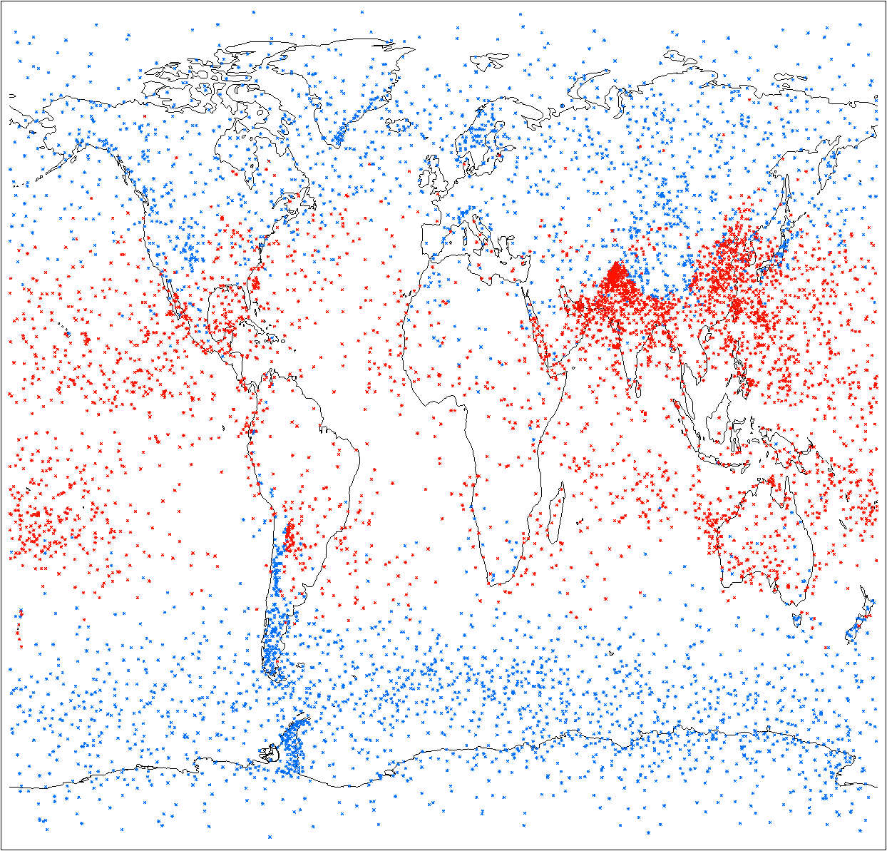

Fig. 2

Distribution of (a) total column water vapor, (b) surface temperature for atmospheric profiles in the dataset.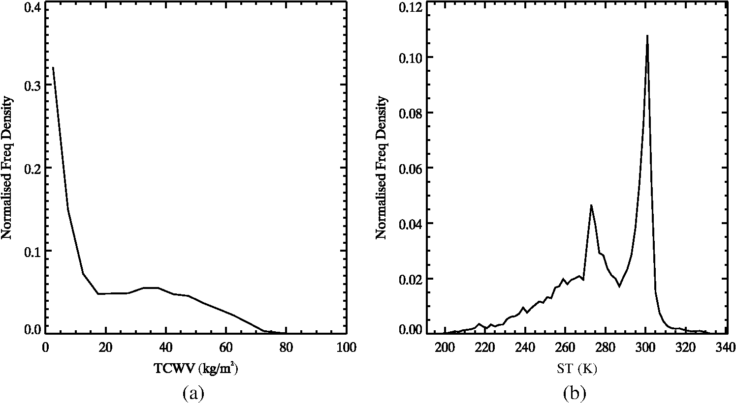

Table 1

The number of atmospheric profiles in each group.

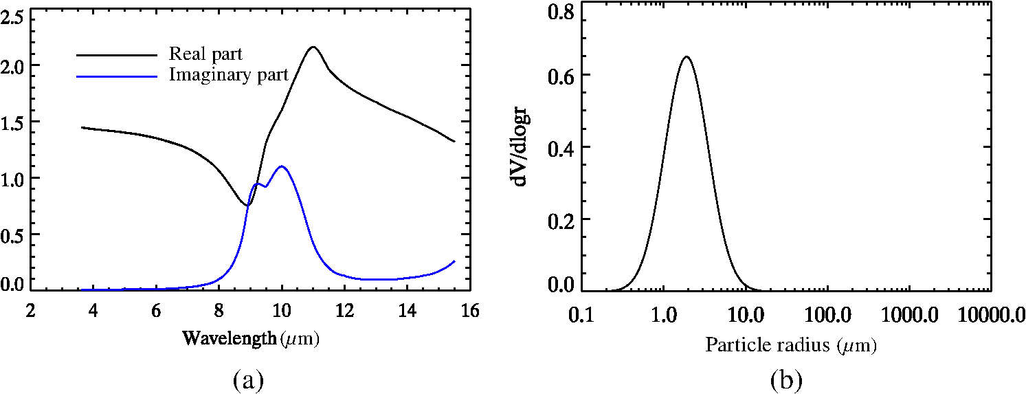
The radiative transfer model RTTOV v11²⁸ was used to simulate brightness temperatures (BTs) observed by the SEVIRI sensor, both under clear sky conditions and in the presence of volcanic ash. Radiative transfer models simulate the attenuation of radiation emitted from, or reflected by, the surface of the Earth as it travels through the atmosphere to be recorded at the sensor. Ash clouds with a geometric thickness of 1 km, with ash concentrations ranging from 7 to $4000\mu \mathrm{g}/{\mathrm{m}}^3$ were simulated at 1 km intervals for altitudes between 1 and 10 km above the surface. Ash clouds with a geometric thickness of 500 m were also simulated, but the results were not markedly different to those for the 1-km clouds and so are not included here (this is not surprising since observations are sensitive to the column loading of ash rather than to the volumetric concentration—by using a fixed geometric thickness here, changes to the concentration are equivalent to changes to the column loading). The difference between the observations simulated for ash from a specific atmospheric profile and those simulated for clear sky using the same profile can be viewed as the sensitivity of the satellite observation to the presence of volcanic ash in that particular atmosphere, i.e., the ash signal modeled for that atmospheric profile.

Observations were simulated for channels centered at 10.8 and $12.0\mu \mathrm{m}$, and both the single channel signal at $10.8\mu \mathrm{m}$ and the BTD signal were calculated, $\mathrm{BTD}=\mathrm{BT}(10.8\mu \mathrm{m})-\mathrm{BT}(12.0\mu \mathrm{m})$.

The signal is calculated for every ash cloud in every atmospheric profile. This means that many signals are calculated within each atmospheric group—corresponding to the different ash cloud altitudes, concentrations, and atmospheric profiles modeled within each group (the atmospheric groups are listed in Table 1). Within each atmospheric group, the simulated ash signals are grouped according to ash cloud altitude and mass concentration, and the mean and variance is calculated for the signals in each of these subgroups. This provides the altitude- and concentration- dependent mean ash signal and its variance for each atmospheric group.

The mean signal is plotted as a function of ash concentration and altitude to demonstrate whether a clear relationship exists between it and the ash concentration and to examine to what extent the altitude of the ash affects this relationship. The variance of the signal is also plotted as a function of ash concentration and altitude. This would be near zero everywhere if only the ash affected the signal (since the only differences between the simulations for a specific ash concentration and altitude are the atmospheric profiles in which the ash is modeled). The variance is, therefore, a measure of the sensitivity of the ash signal to nonash atmospheric effects. Nonzero values for the variance indicate that ash at that particular altitude, with that particular concentration, appears differently in IR observations when it is present in a different atmospheric column. A high variance in the ash signal modeled for a given concentration and altitude implies that the signal is highly sensitive to the atmospheric effects, while a narrow range implies that atmospheric effects can be largely ignored since this would show that the signal is not strongly affected by atmospheric effects and is likely to be more sensitive to properties of the ash such as mass concentration.

The optical properties used to simulate the ash observations, which are based on a lognormal PSD and the complex refractive indices measured for andesite by Ref. 29, see Fig. 3. The Pollack measurements for andesite have been used for interpretation of satellite observations of volcanic ash in other works;^16,30 however, the composition of volcanic ash varies between eruptions and IR observations are known to be sensitive to this¹¹ and to the PSD of the ash grains.¹⁶ The PSD used here is a fit to observations recorded by aircraft following the eruption of Eyjafjallajökull in 2010.³¹ This study is not an investigation into the sensitivity of observations to these properties, but rather into the sensitivity of observations to atmospheric effects, and so it is appropriate that they remain fixed. It should be noted, however, that we have not investigated how the sensitivity of observations to atmospheric effects changes with ash composition or PSD. The results presented here, therefore, may not reflect sensitivity to atmospheric effects for IR observations of ash with a nonandesitic composition or with a different PSD.

Fig. 3

Assumptions made for calculation of the optical properties of volcanic ash. (a) Complex refractive indices presented in Pollack (1973) for andesite and (b) particle size distribution.

3.

Results

Passive observations from space-borne instruments are generally more sensitive to total column amounts of ash than to concentration by volume, as a dense but geometrically thin ash cloud may appear indistinguishable from a sparse geometrically thick cloud when viewed from directly above. Thus the results are presented here in terms of the total column amount of volcanic ash (all the simulated ash clouds are 1 km thick and so the concentration, in $\mathrm{g}/{\mathrm{m}}^3$, is simply the total column amount divided by 1000). The lowest ash concentration to trigger a VAAC to be issued is $200\mu \mathrm{g}/{\mathrm{m}}^3$, which corresponds to $0.2\mathrm{g}/{\mathrm{m}}^2$ for a 1-km thick ash cloud. Each of the atmospheric groups listed in Table 1 is plotted separately so that sensitivities can be compared for different types of atmosphere. Figure 4 shows how the mean signal in the $10.8\mu \mathrm{m}$ channel changes with ash concentration and altitude and Fig. 5 shows the same for the BTD signal. Figure 6 is a plot of the variance of the signal, calculated for each concentration and altitude. The variance is a measure of the range of signals produced by the same ash in different atmospheres, even when the atmospheres share similar characteristics and so belong to the same group in Table 1. Figure 7 shows the variance for the BTD signal and how the variance changes with ash concentration and altitude in the different atmospheric groups.

Fig. 4

The mean change in brightness temperature in the Spinning Enhanced Visible and InfraRed Imager (SEVIRI) channel centered at $10.8\mu \mathrm{m}$ for a range of atmospheric profiles that occurs when ash is added [i.e., the brightness temperature (BT) signal for ash]. (a) Day, tropical, land; (b) day, nontropical, land; (c) night, tropical, land; (d) night, nontropical, land; (e) day, tropical, sea; (f) day, nontropical, sea; (g) night, tropical, sea; and (h) night, nontropical, sea.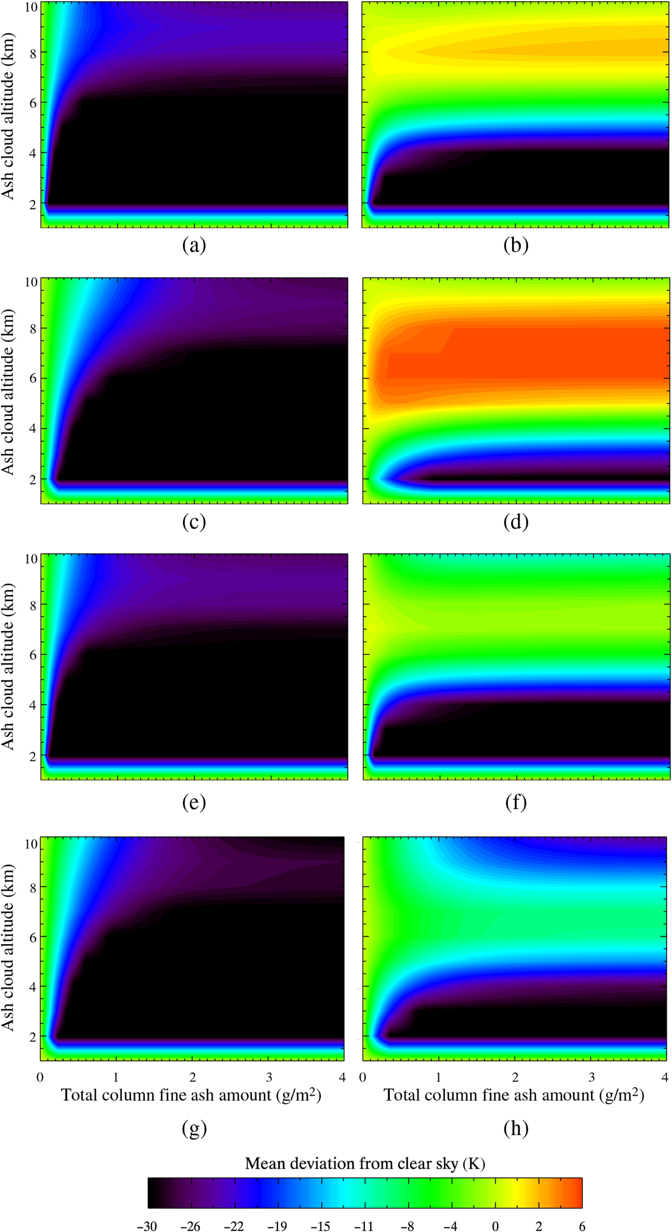

Fig. 5

The mean difference in brightness temperature difference (BTD) (${\mathrm{BT}}_{10.8\mu \mathrm{m}}-{\mathrm{BT}}_{12.0\mu \mathrm{m}}$) for a range of atmospheric profiles that occurs when ash is added (i.e., the BTD signal for ash). (a) Day, tropical, land; (b) day, nontropical, land; (c) night, tropical, land; (d) night, nontropical, land; (e) day, tropical, sea; (f) day, nontropical, sea; (g) night, tropical, sea; and (h) night, nontropical, sea.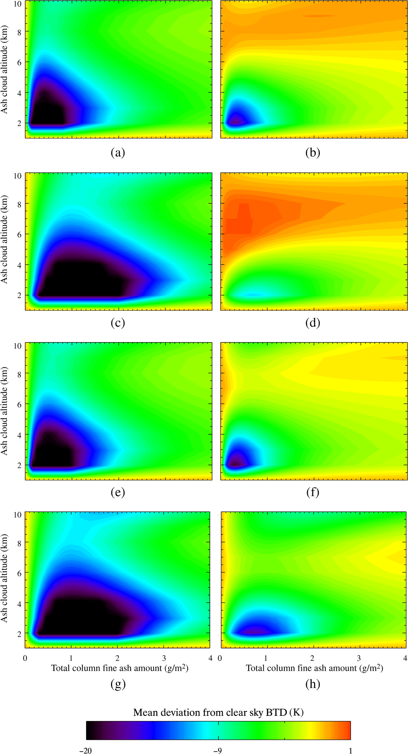

Fig. 6

The variance of the BT signal in the SEVIRI channel centered at $10.8\mu \mathrm{m}$. There are large differences between the variances found for different atmospheric profile groupings, and so individual color scales are used. (a) Day, tropical, land; (b) day, nontropical, land; (c) night, tropical, land; (d) night, nontropical, land; (e) day, tropical, sea; (f) day, nontropical, sea; (g) night, tropical, sea; and (h) night, nontropical, sea.

Fig. 7

The variance of the BTD signal. There are large differences between the variances found for different atmospheric profile groupings, and so individual color scales are used. (a) Day, tropical, land; (b) day, nontropical, land; (c) night, tropical, land; (d) night, nontropical, land; (e) day, tropical, sea; (f) day, nontropical, sea; (g) night, tropical, sea; and (h) night, nontropical, sea.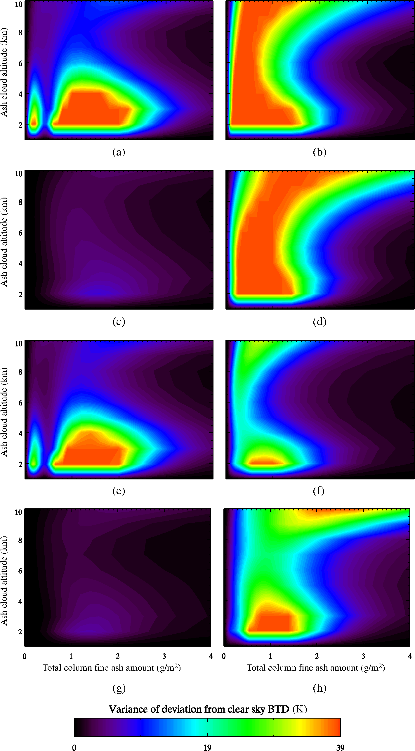

4.

Interpretation and Discussion

The mean plots show the mean signals produced by ash under different atmospheric conditions and show that a different relationship exists between concentration, altitude, and the ash signal when the ash is present in a different type of atmosphere (Figs. 4 and 5). The variance plots indicate the certainty with which the relationships in the mean plots can be assumed to apply to ash when it is present in each type of atmosphere (Figs. 6 and 7). In this section, we discuss each of the figures in turn.

5.

Conclusions

If the altitude, composition, PSD, and concentration of volcanic ash are known, then the effect of the ash on an IR observation of otherwise clear sky cannot generally be predicted without taking into account the specific atmosphere in which the ash is present. The same consideration is, therefore, necessary for interpretation of an observed signal in terms of any of the above properties. The signal produced by the same ash concentration, at the same altitude, with the same composition can vary greatly when the ash is present in an atmosphere with different properties, even if the two atmospheres being compared share similar characteristics. This is particularly the case for ash in nontropical atmospheres over land. The high variance seen for the ash signals investigated here suggests that there exist a range of atmospheric conditions for which interpretation of either of these ash signals without consideration of the imaged atmosphere would be inappropriate, even in conditions where the mean signal is clearly related to ash altitude and/or to concentration. The BTD signal is more consistent and more reliable than the single channel signal, however, the same ash concentration at the same altitude can have a very different effect on the observed BTD when the ash is present in different atmospheric conditions, particularly over land and particularly during the day. The sensitivity of the signals to atmospheric effects varies between tropical and nontropical atmospheres. Interpretation of these signals should be associated with uncertainties that are attributable to atmospheric effects, which are dependent on the characteristics of the imaged atmosphere.

In nontropical atmospheres, and to a lesser extent in tropical atmospheres, the effect of the ash on both the BT in the $10.8\mu \mathrm{m}$ channel and on the observed BTD may be to increase it from the clear sky value. This occurs for some ash concentrations that are considered hazardous in some nontropical atmospheres. Both the altitude of the ash and the properties of the atmosphere in which it is present are required in order to predict the sign of the change affected by the ash to both the single channel and the BTD observations in nontropical atmospheres. Without this information, it is likely that some ash will not be discriminated since it is likely to correspond to a deviation from the observation for clear sky with the opposite sign to that which is expected.

Interpretation of either the single channel or the BTD signal in terms of ash amount is only possible if the altitude of the ash is known, and the properties of the imaged atmosphere, such as water vapor amount and tropopause height, are accounted for. Hazardous ash concentrations may not be identified if these effects are not considered, as “medium” hazard levels of ash may give the same signal as “low” hazard levels of ash if the ash altitude or the properties of the atmosphere are different, even if the atmospheres are similarly “tropical” or “nontropical.”

The BTD and single channel signals for ash can only be interpreted in terms of ash concentration if the ash altitude is known, and the high variance in both signals evident in most atmospheric conditions for nearly all altitudes shows that ignoring atmospheric effects could lead to very high uncertainties associated with such interpretations. Since the properties of the ash modeled for calculation of the signal mean and variance were identical, the spread seen in the signals is wholly attributable to atmospheric effects. It should, therefore, be possible to reduce uncertainties by accounting for the imaged atmosphere, for example, from numerical weather predictions for the scene.