1.

Introduction

There has been an increase in trees and shrubs on rangeland systems in the past 150 years.^1–3 This increase in woody species comes at the expense of perennial grasses whose losses can cause changes in primary production, nutrient cycling, and the accumulation of soil organic matter.⁴ In order to decrease the loss of inherent ecosystem function, vegetation mortality, and increased runoff associated with rangeland system degradation, it is necessary to utilize effective conservation practices. One such practice is brush management, which typically employs prescribed burning, mechanical methods (e.g., chaining, roller chopping, root plowing, shredding, and bulldozing), chemical methods (i.e., herbicide application), or a combination of these methods to control unwanted woody vegetation.⁵ Between 1997 and 2003, the United States Department of Agriculture’s (USDA) Natural Resources Conservation Service (NRCS) spent nearly $34 million dollars on conservation practices, over $19 million being for brush management alone, on 188 million ha of central and western rangelands and grazed forests.⁶ With such a large investment of resources being allocated toward the implementation of brush management, it is essential to have a mechanism for evaluating its effectiveness. The cost combination of labor, equipment, vehicles, travel, and supplies, make traditional ground-based methods of data collection on large scales prohibitively expensive. A pilot study to sample 400 sites (800 points) on 3.1 million ha of rangeland and pinyon-juniper woodlands, reported costs of sampling 448 points by 12 people working 10–12 h per day (data collection and travel) from early June to mid-October at approximately $400,000, with field data collection cost before analysis, averaging $893 per sample point.⁷ Evaluating nearly 200 million ha solely using on-the-ground resources is simply not feasible. A new large-area method is required.

Due to its ability to provide information faster and more cost-effectively than ground-based data collection, remote sensing has been used to map, monitor, and assess vegetation over large areas for over 30 years.^8–17 Within the last 10 years, new government programs, policy changes, and technological advances have made remotely sensed data more accessible than ever before. The USDA Farm Service Agency’s (FSA) National Agriculture Imagery Program (NAIP) has been collecting and providing free, publically available, high-resolution aerial imagery for the continental United States since 2003. Further, the global, multidecadal Landsat satellite data record (1980s to present), together with Landsat’s free data policy, make county, state, regional, and national scale vegetation assessment possible. There was a time when cost made the use of remotely sensed products for long-term monitoring purposes unrealistic. However, with the availability of these no-cost, high spatial, and high temporal resolution datasets, remotely sensed assessment of the effectiveness of conservation practices that strongly influence vegetation cover (e.g., brush management) is now attainable.

Remote sensing has been used to assess woody vegetation in arid and semiarid rangeland systems around the world.^8,18–24 Assessments are commonly performed using spectral mixture modeling^{18,19,25–29} and land cover maps^{20–22,24,30} produced through supervised classification techniques. These methods often employ the use of high-resolution ($<15\mathrm{m}$) satellite imagery, aerial photography, or hyperspectral data. However, the nature of these methods does not easily lend itself to operational use. High-resolution imagery is often expensive to obtain, not readily available on an extended temporal basis, and the requirements that attend its use (e.g., software and skilled labor for data preprocessing, development of image processing algorithms, and data management and storage) present additional challenges. Likewise, resource investments (people, time, money, and equipment) for collection of the data required for ground-truth land cover maps are often prohibitive for repetitive map production. To be of practical use by land managers, the quantification of large-scale woody vegetation cover must be possible using a fairly straightforward and easy to apply methodology that utilizes inexpensive (free) imagery and requires minimal image processing (due to time constraints of overburdened personnel). Thus, the objective of this study was to develop an operationally oriented method for assessing woody vegetation cover using publically available, no-cost remotely sensed data sources on semiarid rangelands in southeastern Arizona.

2.

Methodology and Data Processing

The goal of this work was to develop an operational remote sensing protocol for quantifying woody vegetation cover using no-cost imagery. This protocol is intended for use by land managers to aid in implementing, monitoring, and assessing the effects of brush management conservation practice applications. The woody species Prosopis L. (mesquite) was the focus of this particular study. Sections 2.1–2.3 include descriptions of the study areas, ground-based datasets, imagery used, its processing, the integration process used for subpixel discernment of woody vegetation, and the generation of the relation to quantify woody cover.

2.1.

Study Areas

The study was conducted within major land resource area (MLRA)-41 Southeastern Arizona Basin and Range³¹ and on the Empire Ranch in southeastern Arizona (Fig. 1). The Arizona portion of MLRA-41 covers approximately $\mathrm{36,281}{\mathrm{km}}^2$. Elevation ranges from 975 to 1525 m and the average annual precipitation ranges from 304 to 406 mm with 60% of the rainfall occurring between July and September. The Empire Ranch, which is operated by the Bureau of Land Management (BLM), is located within the Las Cienegas National Conservation Area in the Sonoita Valley of southern Arizona. It is a high profile multiple use area which includes BLM, Pima County, State Trust, and private lands. The ranch is managed cooperatively with significant citizen input, is actively used for cattle ranching, and has experienced a number of conservation management practices (prescribed grazing, prescribed burning, and mechanical grubbing for brush removal). The dominant vegetation is native grass, including Bouteloua gracilis (Willd. ex Kunth) Lag. ex Griffiths (blue grama), Bouteloua eriopoda (Torr.) Torr. (black grama), Bouteloua curtipendula (Michaux) Torr. (sideoats grama), Bouteloua hirsuta (Lagasca) (hairy grama), and Aristida spp. Woody species are mainly comprised of Prosopis L. (mesquite) and Populus L. (cottonwood).

Fig. 1

Major land resource area 41 overlaid with a Landsat-5 TM tile for path 35, row 38, and the Empire Ranch study area with National Agricultural Imagery Program (NAIP), National Resources Inventory (NRI), The Nature Conservancy (TNC), brush removal, and Empire Ranch sampling block (${\mathrm{ER}}_{\text{BLOCK}}$) study sites. NAIP and NRI represent high-resolution imagery subset locations. TNC and ${\mathrm{ER}}_{\text{BLOCK}}$ represent ground-based sampling locations.

Mechanical grubbing for brush removal was performed at several locations on the Empire Ranch. Brush removal treatments occurred from October 18, 2010 to January 26, 2011 on three sites covering approximately 180 ha (Fig. 1). These sites were used to conduct a pre- and post-treatment assessment of woody cover.

2.2.

Data Collection and Processing

Five years of pre-existing ground-based data collected on the Empire Ranch and at National Resources Inventory (NRI) sites within the MLRA were used for the study (Table 1). The NRI and Empire Ranch sampling block (${\mathrm{ER}}_{\text{BLOCK}}$) data were collected by NRCS and USDA Agricultural Research Service Southwest Watershed Research Center personnel, respectively. The Nature Conservancy (TNC) data were collected by TNC employees and volunteers as part of an annual monitoring program for the Empire Ranch. The line-point intercept³² method was used to measure foliar canopy cover by species at all locations. Only woody species cover data were used for analysis. Five years of remotely sensed data were also obtained for the study (Table 2). The datasets NRI, NAIP, and Landsat-5 thematic mapper (TM) imagery were used for training, validation, and equation development. Descriptions of image selection criteria and processing procedures are provided in subsections 2.2.1–2.2.3.

Table 1

Ground-based dataset description. NRI=National Resources Inventory, TNC=The Nature Conservancy, ERBLOCK=Empire Ranch sampling block.

Dataset (number of points)	Collection year	Plot size (m)	Transect length (m) (number of lines)
${\mathrm{NRI}}_{04}$ (7)	2004	$50\times 50$	46 (2)
${\mathrm{TNC}}_{06}$ (16)	2006	$50\times 100$	50 (10)
${\mathrm{TNC}}_{08}$ (15)	2008	$50\times 100$	50 (10)
${\mathrm{TNC}}_{12}$ (12)	2012	$50\times 100$	50 (10)
${\mathrm{ER}}_{\text{BLOCK}\_1}$ (1)	2011	$80\times 80$	60 (6)
${\mathrm{ER}}_{\text{BLOCK}\_2}$ (1)	2011	$50\times 30$	50 (5)
${\mathrm{ER}}_{\text{BLOCK}\_3}$ (1)	2011	$100\times 100$	60 (6)
${\mathrm{ER}}_{\text{BLOCK}\_4}$ (1)	2012	$80\times 80$	60 (4)
${\mathrm{ER}}_{\text{BLOCK}\_5}$ (1)	2012	$80\times 80$	60 (4)

Table 2

Imagery dataset description. NRI=National Resources Inventory, NAIP=National Agricultural Imagery Program, TM=Landsat-5  Thematic Mapper.

Type of image	Acquisition date	Purpose of use
${\mathrm{NRI}}_1$	August 23, 2002	Equation development
${\mathrm{NRI}}_2$	August 23, 2002	Equation development
${\mathrm{NRI}}_3$	August 23, 2002	Equation development
${\mathrm{NRI}}_4$	August 23, 2002	Equation development
${\mathrm{NRI}}_5$	August 23, 2002	Equation development
${\mathrm{NAIP}}_{\mathrm{P}1}$	August 07, 2013	Training, validation
${\mathrm{NAIP}}_{\mathrm{P}2}$	August 07, 2013	Training, validation
${\mathrm{NAIP}}_{\mathrm{C}1}$	July 23, 2013	Training, validation
${\mathrm{NAIP}}_{\mathrm{C}2}$	July 23, 2013	Training, validation
TM	June 17, 2006	Validation
TM	June 22, 2008	Validation
TM	June 15, 2011	Validation, equation development

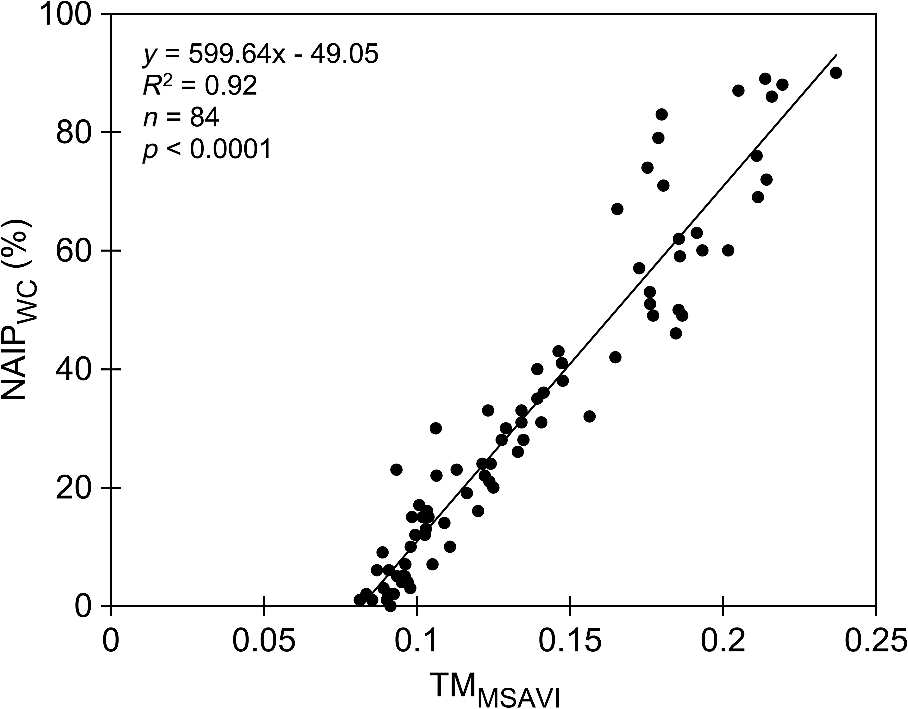
It should be noted that dataset acquisition dates ranged from 2002 to 2013. However, barring the occurrence of major disturbance (e.g., mechanical removal, fire), mesquite cover changes very slowly ($<1\%$ per year) in the Southwest.^33–35 Given that no disturbance events occurred within the areas examined for this study, the assumption was made that comparisons made of datasets acquired within a 3-year window of one another were valid.

2.2.1.

National Resources Inventory imagery

The NRCS rangeland NRI image scenes are ultra-high-resolution (0.305-m), three-band (red, green, and blue) aerial photographs that have been collected as part of the NRI^36,37 data collection efforts since 2000. Five scenes were used for the study (Table 2). Each scene covered approximately $1609{\mathrm{m}}^2$ and was subset to correspond with ground data collection sites. All subsets were classified as woody or nonwoody through supervised object-oriented classification performed with Overwatch Systems LTD’s Feature Analyst^®. Object-oriented analysis utilizes both the spectral characteristics of pixels and their spatial arrangement.²⁴

2.2.2.

National Agriculture Imagery Program imagery

Three-band (red, green, and blue) mosaicked NAIP images for Pima (${\mathrm{NAIP}}_{\mathrm{P}}$) and Cochise (${\mathrm{NAIP}}_{\mathrm{C}}$) counties collected on August 07, 2013, and July 23, 2013, respectively, were obtained from the USDA NRCS Geospatial Data Gateway.³⁸ The NAIP scenes were 1-m ground sample distance ortho-imagery rectified within $\pm 6\mathrm{m}$ to true ground at a 95% confidence level and formatted to a UTM NAD83 coordinate system. Subsets of the images (${\mathrm{NAIP}}_{\mathrm{P}1}$, ${\mathrm{NAIP}}_{\mathrm{P}2}$, ${\mathrm{NAIP}}_{\mathrm{C}1}$, and ${\mathrm{NAIP}}_{\mathrm{C}2}$) were selected to represent vegetation found in the mesquite grassland portions of the TM tiles (Fig. 2). ${\mathrm{NAIP}}_{\mathrm{P}1}$ and ${\mathrm{NAIP}}_{\mathrm{C}1}$ are examples of grassland areas with low to moderate levels of mesquite. ${\mathrm{NAIP}}_{\mathrm{C}1}$ was more sparsely vegetated with greater soil heterogeneity. ${\mathrm{NAIP}}_{\mathrm{P}2}$ and ${\mathrm{NAIP}}_{\mathrm{C}2}$ are examples of mesquite dominated areas, with ${\mathrm{NAIP}}_{\mathrm{P}2}$ being largely composed of mesquite and the large bunchgrass Sporobolus airoides (Torr.) Torr. (alkali sacaton). All subsets were classified as woody or nonwoody through supervised object-oriented classification performed with Overwatch Systems LTD’s Feature Analyst^®. Accuracy assessments of each scene were performed using error matrices with 100 randomly distributed sample points per class.³⁹

Fig. 2

Examples of NAIP subsets from Pima and Cochise counties collected on August 07, 2013 and July 23, 2013, respectively.

2.2.3.

Thematic Mapper imagery

Moderate-resolution (30 m) TM image tiles of path 35, row 38, selected for the study were downloaded from the USGS Earth Explorer website⁴⁰ and had been atmospherically corrected to surface reflectance using the Landsat Ecosystem Disturbance Adaptive Processing System.^41,42 Scenes came processed to standard terrain correction (level 1T), which provides systematic radiometric and geometric accuracy by integrating ground control points while utilizing a digital elevation model for topographic accuracy. All scenes were converted to UTM North American Datum of 1983 (NAD83) zone 12.

The landscape of MLRA-41 is a mix of heterogeneous vegetative cover and soil types. Therefore, characterizing its vegetation canopies will require the use of a spectral vegetation index that can handle such variability. One of the greatest concerns for assessing the sites used in this study was the influence of soil background conditions, which can have considerable influence on calculated vegetation indices for partial canopy spectra.^43,44 The normalized difference vegetation index (NDVI)⁴⁵

Eq. (1)

$$\mathrm{NDVI}=\frac{\rho \mathrm{NIR}-\rho \mathrm{red}}{\rho \mathrm{NIR}+\rho \mathrm{red}},$$

where $\rho \mathrm{NIR}$ and $\rho \mathrm{red}$ are near-infrared (NIR) and red reflectance, is one of the most commonly used indices for assessing vegetation with remotely sensed data. However, the NDVI is sensitive to optical properties of soil background, particularly when vegetation is sparse, making it problematic for application to data spanning different soil types.^43,45,46 The soil-adjusted vegetation index (SAVI)

Eq. (2)

$$\mathrm{SAVI}=\frac{\rho \mathrm{NIR}-\rho \mathrm{red}}{\rho \mathrm{NIR}+\rho \mathrm{red}+L}(1+L),$$

is capable of minimizing the effects of variable soil backgrounds through the use of an $L$ adjustment factor.⁴³ However, to obtain the most precise measures of SAVI, knowledge of vegetative densities for the area of interest is needed to select the most appropriate value for $L$ (e.g., $L=1$ for very low vegetation densities, $L=0.5$ for intermediate densities, and $L=0.25$ for higher densities).^43,44 This can be an issue when looking at large areas containing varying densities of vegetation. Unlike SAVI, the modified soil-adjusted vegetation index (MSAVI)

Eq. (3)

$$\mathrm{MSAVI}=\frac{2\rho \mathrm{NIR}+1-\sqrt{{(2\rho \mathrm{NIR}+1)}^2-8(\rho \mathrm{NIR}-\rho \mathrm{red})}}{2},$$

requires no prior knowledge about vegetation densities in order to select the best $L$ value. Instead optimal $L$ values are determined based on the present reflectance.⁴⁷ Due to the heterogeneity of the study area, MSAVI was selected for use in this study.

Given that a vegetative index will only provide a general measure of greenness, it was necessary to use phenologic timing to discriminate between woody and nonwoody vegetation canopies. Initial selection of TM scenes for the study was based on a short preliminary study conducted to identify the time period that would provide the greatest contrast between mesquite and herbaceous canopies. Homogeneous areas of mesquite and herbaceous vegetative cover were sampled from cloud-free ${\mathrm{TM}}_{\mathrm{MSAVI}}$ images ranging from January 1, 2002, through December 31, 2011. Mean monthly MSAVI values of the mesquite and herbaceous areas were calculated and plotted for the time series (Fig. 3). Optimal timing for capturing the greatest contrast between the two canopy types was between June and July, with mid- or late- June being most favorable.

Fig. 3

Comparison of MSAVI-based greenness for mesquite and herbaceous canopies over time.

Cloud-free scenes of June were then screened for precipitation. Occurrence of precipitation events was evaluated using data generated from Daymet,⁴⁸ a collection of algorithms and computer software that interpolates and extrapolates from daily meteorological observations to produce gridded estimates of daily weather parameters over large regions at 1-km spatial resolution. Studies in semiarid environments have demonstrated that germination of annual forbs and grasses can begin at precipitation levels ranging from 10 to 25 mm.^49–51 This appearance of green vegetation sparked by winter rains is often followed by a subsequent senescent period.⁵² It is during this senescent period that deep-rooted woody vegetation will green-up, with perennial grasses following after the onset of summer rains (Fig. 3). However, an occurrence of subsequent rainfall events following germination can lead to the presence of a green herbaceous cover extending into the critical window needed for discriminating woody from herbaceous canopies. Moreover, it has been observed that 50.8 mm (2 in.) of winter precipitation can sustain herbaceous vegetation until summer precipitation arrives.⁵³ Therefore, all scenes with a cumulative precipitation (January 1 to the image date) of 50.8 mm or greater were eliminated in an effort to decrease the likelihood that green herbaceous vegetation was present. Finally, TM scene selection was narrowed to years spanning the 2006 to 2011 timeframe to facilitate application with available coincident datasets (Table 2).

2.3.

Subpixel Discernment of Woody Vegetation and Equation Development

Moderate-resolution satellite imagery is useful for examining vegetation cover over large areas. However, when trying to discriminate between vegetation types, the presence of mixed pixels can be problematic. In this study, a method was needed to “unmix” pixels without having to undertake the more complicated methods used for spectral unmixing.^54–57 This was accomplished by integrating moderate 30-m resolution imagery with higher 1-m resolution imagery.

Each classified NAIP subset was aggregated up to 30-m resolution using a script created in MATLAB^® (Fig. 4). The following is a short description of operations performed within the script for each NAIP scene. The 2011 ${\mathrm{TM}}_{\mathrm{MSAVI}}$ and the classified NAIP images were cropped together so that their dimensions ensured each TM pixel region comprised exactly 900 ($30\times 30$) NAIP pixels. The cropped NAIP image was then reclassified using a binary system, with each pixel given a value of one for woody or zero for nonwoody. This binary image was aggregated to 30-m resolution by passing a $30\times 30$ pixel moving window over the image and calculating the percent woody cover per iteration [Fig. 4(c)]. Percent woody cover was calculated using the following equation:

Eq. (4)

$$\text{Percent woody cover}=\frac{{\sum }_{i=1}^n{v}_i}{n}\times 100,$$

where $v_i$ is a reclassified binary pixel value, $n$ is the total number of pixels in the moving window, and NAIP-based woody cover (${\mathrm{NAIP}}_{\mathrm{WC}}$) scenes were produced.

Fig. 4

Process for aggregating 1-m resolution NAIP to 30-m resolution: (a) a section of unclassified 1-m NAIP image, (b) section of 1-m NAIP image classified as woody or nonwoody, (c) sample of binary aggregation calculation of percent woody cover using Eq. (2) for a $5\times 5\mathrm{m}$ moving window where $n=25$, (d) section of classified NAIP aggregated to 30-m resolution.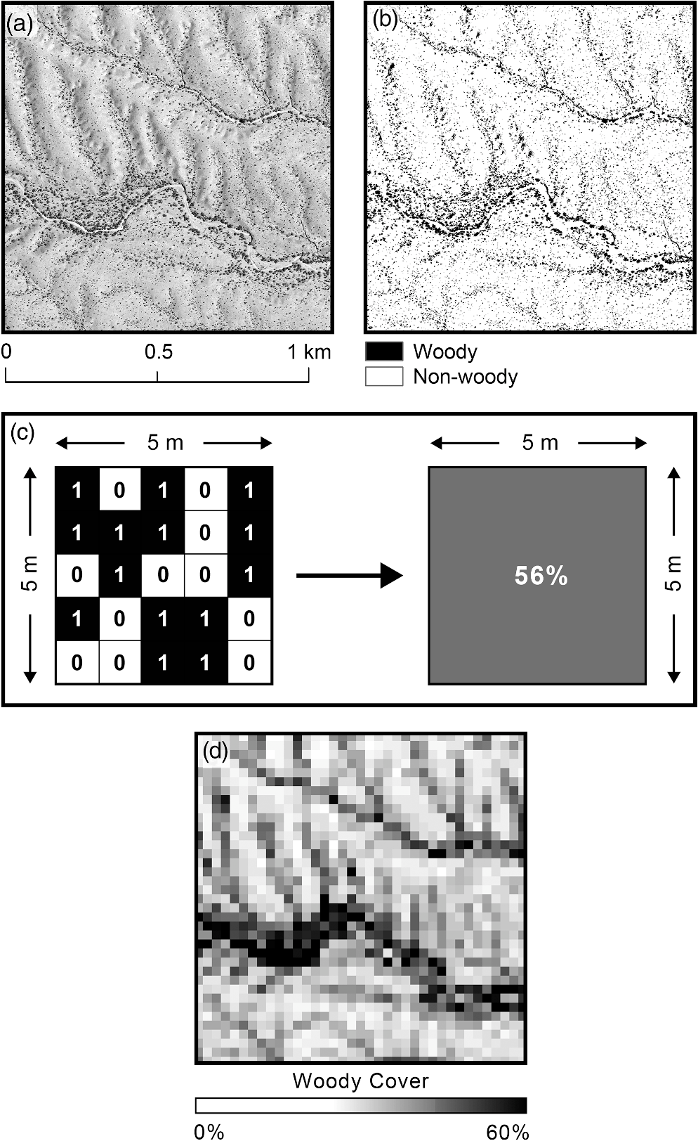

The 2011 ${\mathrm{TM}}_{\mathrm{MSAVI}}$ and ${\mathrm{NAIP}}_{\mathrm{WC}}$ images were used to develop a relationship for producing TM images of woody cover (${\mathrm{TM}}_{\mathrm{WC}}$). A MATLAB script was created to perform randomly stratified sampling of the ${\mathrm{TM}}_{\mathrm{MSAVI}}$ and ${\mathrm{NAIP}}_{\mathrm{WC}}$ scenes. Stratification class bounds were based on the ${\mathrm{NAIP}}_{\mathrm{WC}}$ values (0 to 100%) and set at 10% increments. The number of samples was set to 10 samples per class without replacement. A $3\times 3$ pixel ($90\times 90\mathrm{m}$) window was used for sampling the scenes and the mean ${\mathrm{TM}}_{\mathrm{MSAVI}}$ and ${\mathrm{NAIP}}_{\mathrm{WC}}$ values for the window region were extracted.⁵⁸ The resulting data were split to serve as training and validation datasets. Regression of the training dataset pairs of ${\mathrm{TM}}_{\mathrm{MSAVI}}$ and ${\mathrm{NAIP}}_{\mathrm{WC}}$ was used to develop a relation for ${\mathrm{TM}}_{\mathrm{MSAVI}}$-derived woody cover. The resulting equation was applied to the three ${\mathrm{TM}}_{\mathrm{MSAVI}}$ scenes to create ${\mathrm{TM}}_{\mathrm{WC}}$ scenes. Validation of the ${\mathrm{TM}}_{\mathrm{WC}}$ scenes from 2006, 2008, and 2011 was conducted using the ${\mathrm{NAIP}}_{\mathrm{WC}}$, ${\mathrm{TNC}}_{06}$, and ${\mathrm{TNC}}_{08}$ datasets.

3.

Results and Discussion

The objective of this study was to develop an operationally oriented method for assessing woody vegetation cover using publically available, no-cost remotely sensed data sources on semiarid rangelands in southeastern Arizona. The following is a discussion of the results of the method’s development, including accuracy assessments, validation, and end product usage.

It is often necessary to use pre-existing datasets when conducting large-scale land cover assessments. Traditionally, ground-based measures have been the preferred source of reference data when performing accuracy assessments of remotely sensed products. Unfortunately, ground-based data are not only expensive and time consuming to obtain, but when collected are rarely at a scale appropriate for use with moderate-resolution scenes.^7,36,39 Alternatively, studies^59–62 have used high-resolution airborne imagery as a surrogate for ground-based data. When using this method, a subset comparison of ground-collected and airborne data to verify reliability is recommended.³⁹ Therefore, a comparison of high-resolution image-based woody cover and ground-based woody cover is shown (Fig. 5). Good agreement ($\mathrm{RMSE}=3.8\%$, $\mathrm{MAE}=2.9\%$) was found between the datasets. The error fell within bounds considered reasonable for accepting imagery-based woody cover estimates for use as ground-based surrogates.

Fig. 5

Comparison of high-resolution (NAIP and NRI) imagery-based woody cover and ground-based woody cover. Root-mean-square error (RMSE) and mean absolute error (MAE) are presented.

NAIP imagery was used to produce ground-based woody cover in this study. Accurate classification of this imagery was imperative for generating reasonable estimates of woody cover. Error matrices of the classified NAIP subsets indicated overall accuracies for the subsets that ranged from 93% to 97% (Fig. 6). Misclassification of dark and/or shaded grasses as woody vegetation was a source of error for all subsets. Overclassification of tree clusters was the main source of error for the mesquite dominated scenes (${\mathrm{NAIP}}_{\mathrm{P}2}$ and ${\mathrm{NAIP}}_{\mathrm{C}2}$).

Fig. 6

Error matrices to assess the accuracy of classifications performed on four NAIP subsets of images from Pima (${\mathrm{NAIP}}_{\mathrm{P}1}$, ${\mathrm{NAIP}}_{\mathrm{P}2}$) and Cochise (${\mathrm{NAIP}}_{\mathrm{C}1}$, ${\mathrm{NAIP}}_{\mathrm{C}2}$) counties captured on August 07, 2013 and July 23, 2013, respectively.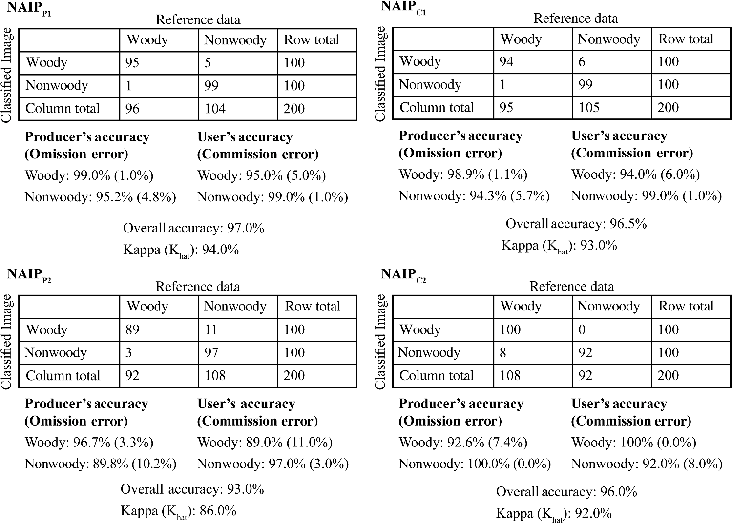

The practice of relating spectral vegetation indices to vegetative properties (e.g., canopy cover, LAI, biomass, leaf water content, and chlorophyll) is well documented.^63–65 In this study, a strong ($R^2=0.92$) linear relationship was found between ${\mathrm{TM}}_{\mathrm{MSAVI}}$ and ${\mathrm{NAIP}}_{\mathrm{WC}}$ (Fig. 7). The resulting equation:

Fig. 7

Relationship of 2013 ${\mathrm{NAIP}}_{\mathrm{WC}}$ to 2011 ${\mathrm{TM}}_{\mathrm{MSAVI}}$. Regression is significant.

Validation is a critical step in the production of remotely sensed products.^39,66,67 Assessment of the 2006, 2008, and 2011 ${\mathrm{TM}}_{\mathrm{WC}}$ scenes revealed a number of factors responsible for the resultant error ($\mathrm{RMSE}=8.5\%$, $\mathrm{MAE}=6.4\%$) (Fig. 8). First, saturation of ${\mathrm{TM}}_{\mathrm{WC}}$ corresponding to the ${\mathrm{NAIP}}_{\mathrm{WC}(\mathrm{P}2)}$ data was likely due to the possible presence of broadleaved woody species mixed with mesquite canopies that were visually undetectable during initial classification efforts. Next, apparent underestimation of ${\mathrm{TM}}_{\mathrm{WC}}$ for ${\mathrm{NAIP}}_{\mathrm{WC}(\mathrm{P}2)}$ data seen in the mid- to high (40% to 85%) range of observed cover was the result of an inflation of ${\mathrm{NAIP}}_{\mathrm{WC}}$ caused by overclassification of tree clusters and dark and/or shaded grasses. Further, ${\mathrm{TM}}_{\mathrm{WC}}$ was overestimated for ${\mathrm{NAIP}}_{\mathrm{WC}(\mathrm{P}2)}$ data within the lower (5% to 25%) range of observed cover. This was largely due to a resulting disconnect due to the ability to visually detect the sacaton in the ${\mathrm{NAIP}}_{\mathrm{P}2}$ scene when determining observed woody cover, and an inability of ${\mathrm{TM}}_{\mathrm{MSAVI}}$ to differentiate between mesquite and sacaton greenness. Given that green-up of sacaton canopies can start as early as April and last past October, discernment from mesquite greenness was simply unfeasible. Finally, uncertainty in cover estimates when ${\mathrm{TM}}_{\mathrm{WC}}$ was less than 10% was largely dependent on how well the woody signal overcame the underlying ground cover signal. Despite the varied nature of these localized errors, the RMSE and MAE of the ${\mathrm{TM}}_{\mathrm{WC}}$ scenes were within acceptable bounds for operational use to quantify large-scale woody cover for brush management decisions.

Fig. 8

Comparison of observed (${\mathrm{NAIP}}_{\mathrm{WC}(\mathrm{P}1)}$, ${\mathrm{NAIP}}_{\mathrm{WC}(\mathrm{P}2)}$, ${\mathrm{NAIP}}_{\mathrm{WC}(\mathrm{C}1)}$, ${\mathrm{NAIP}}_{\mathrm{WC}(\mathrm{C}2)}$, ${\mathrm{TNC}}_{06}$, and ${\mathrm{TNC}}_{08}$) and predicted (2006, 2008, and 2011 ${\mathrm{TM}}_{\mathrm{WC}}$) woody cover. Root-mean-square error (RMSE) and mean absolute error (MAE) are presented.

These large-scale images of woody cover can provide a picture of the spatial distribution of woody cover that is integral in establishing where removal should occur, and in tracking its re-emergence for subsequent removal. For example, subsets of ${\mathrm{TM}}_{\mathrm{WC}}$ scenes of pre and postbrush removal on the Empire Ranch showed a decrease in woody cover from 30% to 60% in 2008 to 10% to 20% in 2011 within areas treated with brush removal (Fig. 9). Changes seen in the area southwest of the treatments where woody cover dropped from roughly 11% to 60% down to 0% to 5% cover were caused by a wildfire on June 01, 2011. The continuation of the Landsat time series through the launch of Landsat-8 will make tracking reemergence within these treatments post-2011 possible.

Fig. 9

Map subsets of ${\mathrm{TM}}_{\mathrm{WC}}$ on the Empire Ranch for June 22, 2008, and June 15, 2011. Brush removal treatment areas are outlined in black. The years of 2008 and 2011 represent pre- and post-treatment, respectively.

4.

Concluding Remarks

An operationally oriented protocol for quantifying woody vegetation cover with no-cost, publically available imagery is needed to aid land managers in implementing, monitoring, and assessing brush management conservation practice applications. This work showed that it was possible to produce viable ($\mathrm{RMSE}=8.5\%$, $\mathrm{MAE}=6.4\%$) maps of woody cover to track the occurrence of brush removal and monitor the presence or lack of subsequent re-emergence. However, there are a number of conditions that must be upheld to achieve valid results. With regard to Landsat image selection, appropriate phenologic timing for capturing the greatest contrast between the woody species of interest and other vegetative cover is critical. Precipitation and cloud cover must also be considered. In this study, the woody species of interest was mesquite and optimal timing was mid- or late- June, with less than 50.8 mm of cumulative precipitation occurring before the cloud-free image date. Use of the protocol in other locations (e.g., Texas, New Mexico, Colorado, etc.) will require new determinations of the optimal timing to allow for greatest contrast between woody and nonwoody vegetation, as well as precipitation conditions that limit the occurrence of green forbs and grasses.

Generation and validation of TM scenes to estimate woody cover from ${\mathrm{TM}}_{\mathrm{MSAVI}}$ requires corresponding image-based woody cover values. Given that these image-based woody cover estimates are calculated from classifying high-resolution imagery, accurate classification of woody versus nonwoody vegetation is essential. Misclassification due to shadowing and clumping of vegetation will manifest as error in the validation of Landsat-based woody cover estimates. Early green-up of herbaceous vegetation will also contribute to misclassification error and should be avoided if possible. The relation for woody cover from MSAVI in this study (Eq. 5) was developed to target mesquite cover. It does detect other woody species; however, to achieve the best results, new relations should be developed for use with woody species like Juniperus L. (juniper) or Populus L. (cottonwood) that have reflective signatures that are very different from mesquite.

This study demonstrated that it was possible to produce a viable method for developing an operationally oriented method for assessing woody vegetation using publically available, no-cost remotely sensed data on semiarid rangelands in southeastern Arizona. Future work will include development of new relationships to better quantify juniper and cottonwood species, as well as test protocol applicability to Landsat-8 imagery and other rangeland locations in the central and western United States.