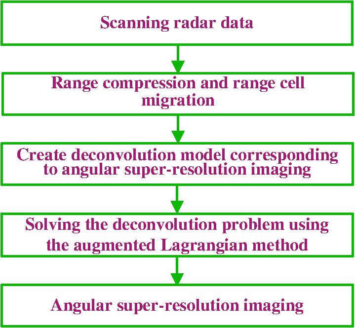
1.

Introduction

Due to advantages over optical sensing tools, such as robust performance under all-time and all-weather circumstances, radar plays an important role in such realms as earth observation, oceanic monitoring, and military reconnaissance.^1,2 To realize these applications, two-dimensional high resolution is usually required. The high range resolution can be obtained by transmitting the wideband signal and using the pulse compression technique. The high resolution in azimuth/angular can be realized using synthetical aperture technique or Doppler beam sharpening approaches. However, these techniques are unable to realize radar imaging in the forward-looking area of the radar platform. The reason is that the Doppler resolution and the range resolution in the forward-looking area are parallel.³

Scanning radar works as a noncoherent sensor, which is suitable for any geometrical situation and is able to realize two-dimensional radar imaging in the forward-looking area of the radar platform. In the same way, the pulse compression provides the high range resolution, while the angular resolution is usually poor when compared with the range resolution. For scanning radar, the upper limit of angular resolution is determined by the effective wavelength and the size of the antenna. Moreover, the angular resolution suffers and degrades as a function of target distance. One method to improve the angular resolution in scanning radar image can be accomplished by increasing the physical size of the antenna aperture. However, there may be insufficient space to accommodate such a large size antenna in the application. Therefore, an improvement in the angular resolution of the scanning radar with fixed parameters using signal processing methods is considered.

According to Refs. 4 and 5, the echo of scanning radar can be modeled as the convolution of the transmitted signal with the scattering coefficients of the targets. Therefore, in theory, a deconvolution method can enhance the angular resolution of the scanning radar.⁶ Deconvolution aims at removing the transfer function, system noise, and other nonidealities of the imaging process, thereby improving the imaging resolution.⁷ The deconvolution approach has been widely used for video restoration,⁸ image processing,⁹ sparse signal restoration,¹⁰ and through-wall radar imaging,¹¹ while less work on the deconvolution approach for angular super-resolution imaging in scanning radar has been reported.

This paper presents a deconvolution method for improving the angular resolution of scanning radar. We first convert the angular super-resolution imaging task in scanning radar into an equivalent deconvolution problem. It is well-known that the deconvolution problem is ill-posed, which means the solution to the deconvolution problem is unstable and sensitive to the noise. To stabilize the solution of the deconvolution problem, we must utilize some prior information of the solution to the deconvolution problem. This paper focuses on some applications such as the detection of detecting and city area imaging, and the case where a small number of dominant scatterers are distributed in the scene. In these applications, large coefficients of the scatterers can capture most of the information of the scene.¹² Inspired by the Bayesian compressive sensing,¹³ the statistic characteristics of the dominant scatterers in the illuminated scene can be represented by $l_1$-norm. Then the deconvolution technique for dominant scatterers in angular super-resolution imaging can be converted into the corresponding $l_1$ optimization problem. Therefore, the $l_1$ regularization is adopted and the deconvolution problem can be written with a constrained optimization form. Recently, applications of $l_1$-norm minimization can be found in Ref. 14 for ISAR imaging,¹⁵ for feature enhanced, and for through-wall radar image.¹⁶ In this paper, we are focused on solving the deconvolution problem, which corresponds to the task of angular super-resolution imaging in the forward-looking area of radar platform. Finally, the constrained optimization problem is solved using an augmented Lagrangian method. The rationale behind the augmented Lagrangian method is to find a saddle point of the associated augmented Lagrangian function, which combines the function to be optimized with a Lagrange multiplier term and a penalty term for the constraints.¹⁷ This leads to an alternating direction method for finding the saddle point of the augmented Lagrangian function. Compared with the traditional Lagrangian multiplier method, the augmented Lagrangian method overcomes numerical difficulties due to the penalty going to infinity.¹⁸ Based on simulation and experimental results, we demonstrate that the proposed deconvolution algorithm has better angular super-resolution performances.

The rest of this paper is organized as follows: Sec. 2 presents the signal model for scanning radar and converts the angular super-resolution problem into an equivalent deconvolution problem. Section 3 presents an augmented Lagrangian method to solve the corresponding deconvolution problem. In Sec. 4, simulation and experimental results are given to demonstrate the validity of the proposed method. Finally, the conclusions are given in Sec. 5.

2.

Signal Model for Scanning Radar in Azimuth

In this section, we introduce the signal model for scanning radar and convert the angular super-resolution problem into an equivalent deconvolution problem. The details of the deconvolution algorithm for the angular super-resolution problem will be subsequently provided.

Suppose that the radar works in the scanning mode. The geometrical model of scanning radar is illustrated in Fig. 1. The radar platform at the altitude $H$ is moving along the $Y$-axis corresponding to the range direction, while the antenna scans the scene along the $X$-axis corresponding to the azimuth direction with constant angular velocity $\omega$ and then receives the echo data from the observed scene. Assume that the target in the azimuth can be considered as an ideal point. For an isolated target scatter, the received signal at the receiver output is proportional to the antenna pattern. The left part of Fig. 1 shows that the scanning radar collects echo data, while it scans in the azimuth across the target field. It is noted that the adjacent echoes mostly cover the same target features on the observed scene but with different contributions to the overall signal, which is shown in the bottom part of Fig. 1.

Fig. 1

The geometrical model of the scanning radar.

At first, the conventional range compression and range migration correction are applied to the echo data with the current approaches.^2,19 The range compression and range migration to correct data are denoted by $g(\theta ,\phi ,r)$, where $r$ is the slant range from the radar to the target and $\theta$, $\phi$ denote the angle between the direction of the antenna to the target and flight direction and the incident angle of the beam, respectively, which are smaller than 10 deg. On the other hand, it is assumed that the antenna pattern is of relative isotropy to the imaging scene. Then the received signal of the scanning radar along the range profile can be recognized as a convolution kernel comprising the antenna power pattern in the angle coordinates and the pulse modulation function in the range dimension,²⁰ which could be expressed as

Without loss of generality, we consider the variation in scattering with the azimuth angle $\theta$ for a fixed range $r_0$ and a fixed angle $\phi$. Note that with the limited range resolution, the range averaging scattering would be exactly equal to the effective scattering evaluated at the range of the interested $r_0$. Thus, we only consider the azimuth variation in Eq. (1) that can be written as

For mathematical simplicity, we only consider the azimuth variation. Then we can rewrite Eq. (2) as

In addition, the presence of the noise contaminates the data $g(\theta )$. The formation of the data $g(\theta )$ can be described as

In the case of observing a certain scene $\mathrm{\Omega }$, the echo returned to the radar is the whole scene. The reflectivity of $\mathrm{\Omega }$ can be denoted as a two-dimensional matrix

To attain the corresponding discrete convolution equation, we represent the scene $\mathrm{\Omega }$ as a vector by stacking the columns of the matrix:

According to Ref. 21, a discrete convolution equation corresponding to Eq. (4) can be written as

The matrix $H$ is a block circulant consisting of circulant blocks with dimensions $RA\times RA$. Each partition of $H_i(i=\mathrm{1,2},\cdots R)$ has the size $A\times A$, which is constructed from the $i$’th scanning antenna pattern. Each partition $H_i$ can be written as

The goal of angular super-resolution in scanning radar is to infer $f$ from the $g$, as accurately as possible. This task is called the deconvolution problem in this paper. The challenge is that the data $g$ recorded at the output of the radar system are a low-pass-filtered version of the original data $f$ due to the “low-pass” filtering effect of the antenna. So the high-frequency parts of the $g$ are lost by the antenna, which leads to the decrease of the azimuth resolution of the scanning radar system.

3.

Augmented Lagrangian Solver for Angular Super-Resolution Imaging

In this section, we first analyze the phenomenon of noise amplification in the conventional inverse filter methods for solving a deconvolution problem. The deconvolution problem is converted into a constrained optimization task. Then the augmented Lagrangian method is presented as the foundation of the following deconvolution method. Finally, the angular super-resolution is realized by solving the constrained optimization via augmented Lagrangian method.

3.3.

Applying Augmented Lagrangian Method to Deconvolution Problem

Starting from Eq. (14), we introduce auxiliary constraint variables $u$ and $v$. The unconstrained optimization problem [Eq. (14)] can be written in the form of Eq. (17) as

Eq. (19)

$$\begin{gathered} {\theta }_1(f)=\lambda {\Vert Lf\Vert }_1 \\ {\theta }_2(Hf)=\frac{1}{2}{\Vert g-Hf\Vert }_2^2 \\ u=Hf,v=Lf. \end{gathered}$$

The unconstrained optimization problem is

Eq. (20)

$$\begin{gathered} \underset{f,u,v}{\arg \min }\{E(f,u,v)=\lambda {\Vert v\Vert }_1+\frac{1}{2}{\Vert g-u\Vert }_2^2\} \\ \text{subject to}:u=Hf,v=Lf. \end{gathered}$$

The authors of Refs. 27 and 29 have also utilized this method in the context of imaging restoration. However, our emphasis here is on angular super-resolution in scanning radar. Before processing, we rewrite Eq. (17) concisely as

Eq. (21)

$$\begin{gathered} \underset{z}{\arg \min }E(z) \\ \text{subject to}:z=Cf, \end{gathered}$$

where $z=\left[\begin{array}{c}u\\ v\end{array}\right]$ and $C=\left[\begin{array}{c}H\\ L\end{array}\right]$. Since Eq. (21) is equivalent to Eq. (14), solving Eq. (21) with respect to $f$ yields the desired radar image with angular super-resolution.

The augmented Lagrangian equation associated with Eq. (21) is

Eq. (22)

$$L_A(f,z,\gamma )=E(z)+{\gamma }^T(z-Cf)+\frac{\mu }{2}{\parallel z-Cf\parallel }_2^2,$$

which combines a multiplier term ${\gamma }^T(z-Cf)$ with Lagrangian multipliers $\gamma \triangleq {[{\gamma }_u^T,{\gamma }_u^T]}^T$ and a quadratic penalty term $\mu /2{\Vert z-Cf\Vert }_2^2$.²⁸ For easier manipulation, the multiplier term can be absorbed into the penalty term in Eq. (22), which leads to the following equation:

Eq. (23)

$$\begin{array}{c}{L}_A(f,z,\gamma )=E(z)+\frac{\mu }{2}{\Vert z-Cf-\eta \Vert }_2^2+\text{const}\end{array},$$

where $\eta \triangleq {[{\eta }_u^T,{\eta }_v^T]}^T=(-1/\mu )\gamma$ is a constant independent of $f$ and $z$, and $\text{const}=(-\mu /2){\Vert \eta \Vert }_2^2$.

Next, we find the saddle point of Eq. (23) using the alternating direction method shown in Table 1, which results in the following equations:

Eq. (24)

$$f_{k+1}=\underset{f}{\arg \min }{\parallel z_k-Cf-{\eta }_k\parallel }_2^2,$$

Eq. (25)

$$z_{k+1}=\underset{z}{\arg \min }E(z)+\frac{\mu }{2}{\parallel z-C{f}_{k+1}-{\eta }_k\parallel }_2^2,$$

Eq. (26)

$${\eta }_{k+1}={\eta }_k-(z_{k+1}-C{f}_{k+1}).$$

We now solve these equations one by one.

3.3.1.

f-subproblem

By dropping the index $k$, the solution of Eq. (24) is found by considering the normal equation as follows:

Eq. (27)

$$C^{T}Cf=C^T(z_k+{\eta }_k),$$

or, equivalently,

Eq. (28)

$$(H^{T}H+L^{T}L)f=H^T[u_k+{({\eta }_u)}_k]+[v_k+{({\eta }_v)}_k].$$

The convolution matrix $H$ in Eq. (28) is a Block Toeplitz matrice, with each element of it being the Toeplitz block structure. This leads to an efficient solution for Eq. (28) using the preconditioned conjugate gradient method. Therefore, Eq. (28) has the following solution:

Eq. (29)

$$f={\mathfrak{F}}^{-1}\left\{\frac{\mathfrak{F}{(H)}^T\mathfrak{F}[u_k+{({\eta }_u)}_k]+\mathfrak{F}[v_k+{({\eta }_v)}_k]}{\mathfrak{F}{(H)}^T\mathfrak{F}(H)+\mathfrak{F}{(L)}^T\mathfrak{F}(L)}\right\},$$

where $\mathfrak{F}$ represents the Fourier transform operator. The matrix $\mathfrak{F}(H)$ can be precalculated outside the main loop. In application where a high number of data are collected, the computation burden of the method is primarily determined by how Eq. (29) is solved, which in turn requires only one forward FFT and one inverse FFT per iteration. Therefore, at each iteration, the main complexity of solving Eq. (28) is in the order of $\mathcal{O}(AR\log A)$ operations.

3.3.2.

z-subproblem

We see that due to the structure of $E(z)$ and $C$, Eq. (25) can be separated into the following parts:

Eq. (30)

$$u_{k+1}=\underset{u}{\arg \min }\{\frac{1}{2}{\Vert g-u\Vert }_2^2+{({\gamma }_u^T)}_k(u-H{f}_{k+1})+\frac{\mu }{2}{\Vert u-H{f}_{k+1}\Vert }_2^2\},$$

Eq. (31)

$$v_{k+1}=\underset{v}{\arg \min }\{\lambda \Vert v{\Vert }_1+{({\gamma }_v^T)}_k(v-f_{k+1})+\frac{\mu }{2}{\parallel v-f_{k+1}\parallel }_2^2\}.$$

Equations (30) and (31) are independent of each other and can be solved simultaneously. Equation (30) is quadratic and has a closed solution.

Eq. (32)

$$u_{k+1}={(1+\mu )}^{-1}[\mu H{f}_{k+1}+g-{({\eta }_u)}_k].$$

According to Ref. 30, Eq. (31) can be solved using the shrinkage equation. Then, Eq. (31) becomes

Eq. (33)

$$\begin{gathered} v_{k+1}={\text{shrink}}_{\frac{\lambda }{\mu }}[v_k-f_{k+1}-{({\eta }_v)}_k] \\ =\frac{v_k-f_{k+1}-{({\eta }_v)}_k}{{\Vert v_k-f_{k+1}-{({\eta }_v)}_k\Vert }_2}\times \max \{{\Vert v_k-f_{k+1}-{({\eta }_v)}_k\Vert }_2-\frac{\lambda }{\mu },0\}, \end{gathered}$$

where $0·(0/0)=0$ is assumed.

Finally, the parameter ${\eta }_u$ and ${\eta }_v$ are updated as

Eq. (34)

$${({\eta }_u)}_{k+1}={({\eta }_u)}_k-(u_{k+1}-H{f}_{k+1}),$$

Eq. (35)

$${({\eta }_v)}_{k+1}={({\eta }_v)}_k-(v_{k+1}-f_{k+1}).$$

To make this clear, the main flowchart of the proposed decovolution algorithm for angular super-resolution in scanning radar is shown in Fig. 2.

Fig. 2

The flowchart of the presented deconvolution algorithm for angular super-resolution imaging.

4.

Experimental Results

In order to show the validity of the proposed deconvolution method for angular super-resolution in scanning radar, simulation and experimental results are presented in this section.

4.1.

Simulations

In this section, the simulation results are presented to demonstrate the performance of the proposed deconvolution method for angular super-resolution in scanning radar. The simulation scene is shown in Fig. 3. The results are compared with those obtained by the Wiener filter method and the operator $L$ is chosen as the $I$, where $I$ represents the identity matrix. In the tests, the iteration was manually adjusted to yield the best angular super-resolution result for each experimental condition. To get the final result of the solution, the parameter $\mu$ is essential. The issue of how to optimally select $\mu$ is important, but is outside of the scope of this work. In this paper, the parameter is set as 10 for all simulations and experiments according to the method from the authors of Ref. 31.

Fig. 3

Simulation scene.

Some related scanning radar system parameters are set as follows: the radar carrier frequency is 10 GHz and the pulse repetition frequency is 4000 Hz with an antenna scanning speed $20\mathrm{deg}/\mathrm{s}$. The bandwidth of the transmitted signal is 2 MHz and the 3-dB width of the real beam is about 3 deg.

In order to quantify and compare the angular super-resolution performance of the proposed deconvolution method on the simulation data, relative error (ReErr),³² structure similarity (SSIM),³³ and the peak-to-valley point difference in decibels are used in the simulations. They are defined as follows:

Eq. (36)

$$\mathrm{ReErr}=\frac{{\parallel \widehat{f}-f\parallel }_2}{{\parallel f\parallel }_2};\mathrm{SSIM}=\frac{2{\rho }_{(\widehat{f},f)}·(2{\mu }_{\widehat{f}}·{\mu }_f)}{({\mu }_{\widehat{f}}^2+{\mu }_f^2)({\sigma }_{\widehat{f}}^2+{\sigma }_f^2)},$$

where $\mu$, $\sigma$, and $\rho$ are the mean, standard deviation of the vectors, and the correlations corresponding to the vectors $f$ and $\widehat{f}$. $\widehat{f}$ and $f$ represent the obtained angular super-resolution result and the original targets, respectively. The SSIM is a quality measurement between the super-resolution result and the original scene. The value of SSIM is between $-1$ and 1, and 1 denotes full identification with the original scene. The peak-to-valley point difference in decibels is defined in Fig. 4 and quantifies the ability of an angular super-resolution algorithm to separate two closely spaced targets. The difference of the peak-to-valley point in decibels is between 0 and $-\infty$, where 0 means that the angular super-resolution algorithm can fully separate two closely spaced targets.

Fig. 4

The definition of the peak-to-valley point difference in decibels.

In order to show the angular super-resolution performance of the proposed method, we simulate the case of different signal-to-noise ratios (SNRs). Figure 5 shows the angular super-resolution results by using the proposed method and Wiener filter approach under different noise levels. Figure 6 shows the evolution of the ReErr and the SSIM with different SNRs. Some observations can be made based on the results in Figs. 5 and 6. For the isolated target, the echo is proportional to the antenna pattern. The echo of two adjacent targets is added and form a single peak as illustrated in Fig. 5. Hence, the individual response cannot be distinguished. The second row of Fig. 5 is the angular super-resolution results obtained by the Wiener filter method, and the third row of Fig. 5 represents the angular super-resolution results given by the proposed deconvolution method. In Fig. 6, the ReErr, whose ideal value is 0, is shown. When the value of the ReErr gets smaller, the precision of the angular super-resolution method increases. The metric SSIM is a quality measurement between the angular super-resolution result and the original scene. The value of SSIM is between $-1$ and 1, where 1 means the angular super-resolution result that fully identifies with the original scene. This leads to the larger value of the SSIM and a better performance of the proposed angular super-resolution method in terms of quality. It is clear that the proposed deconvolution method gives better results than the Wiener filter method. For example, in the case of $\mathrm{SNR}=10\mathrm{dB}$, the angular super-resolution result of our method not only seems more appealing, but also has a better performance in terms of ReErr and SSIMs.

Fig. 5

The results of the angular super-resolution. From top to bottom, you can see the received echo under different Gaussian noise levels and the angular super-resolution results obtained using the Wiener filter and the proposed method, respectively: (a) the noise level is 20 dB; and (b) the noise level is 10 dB.

Fig. 6

Evolution of the ReErr and SSIM along the noise SNRs for the simulations.

4.2.

Experimental Results

In order to show the effectiveness of the proposed deconvolution algorithm for angular super-resolution in scanning radar, the real data results are presented. Figure 7 shows the three buildings and their distributions. The range between the scene center and the radar is about 594 m and the distance of each building is 45 m. The transmitted antenna pattern is obtained through the measurement result in the microwave anechoic chamber in the University of Electronic Science and Technology of China. However, due to the noise and energy degradation in actual situations, the antenna pattern used in deconvolution is not consistent with the transmitted pattern. To achieve nice results, we use a pretreatment for the antenna pattern which changes the length of the sidelobe while retaining the width of the main beam of the original pattern. The width of the sidelobe is changed step by step and is chosen by the best experiment result for random data in one scan. In our experiment for scene data processing, this method for choosing the appropriate antenna pattern is effective. The echo from the three buildings is much stronger than that from other areas so that the scene can be considered as the combination of three point targets. Employing the scanning radar system in Fig. 8, the data are acquired. The scanning radar system parameters for the experiment are listed in Table 2.

Fig. 7

The tested scene.

Fig. 8

The scanning radar system [(a) front side and (b) back side] utilized to collected scattering data.

Table 2

Experimental parameters for real data.

Parameters	Value	Units
Carrier frequency	10	GHz
Bandwidth	30	MHz
Pulse duration	2	$\mu \mathrm{s}$
Pulse repetition frequency	200	Hz
Antenna scanning velocity	70	$\mathrm{deg}/\mathrm{s}$
Antenna scanning area	$-45$ to $+45$	deg
Main-lobe beam width	5	deg

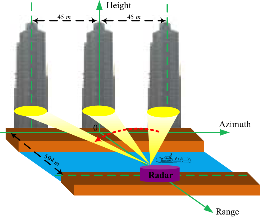
Compared with the Wiener filter result, the proposed method yields a greater radar image quality with increased resolution, as shown in Fig. 9. Different rows in Fig. 9 correspond to the imaging result with the azimuth profile of the target scene. The first row of Fig. 9 shows the scanning radar image. The image cannot distinguish the positions of the buildings. Compared with the second row of Fig. 9, the third row shows the improved angular resolution and higher visual quality. The reason is that the prior information of the target is used in the proposed method, while the Wiener filter method uses no prior information of targets. Therefore, the proposed method is more effective compared with the Wiener filter method.

Fig. 9

Radar imaging results of real data: (a) the scanning radar image and the azimuth profile of the target area, respectively. (b) The angular super-resolution imaging result via the Wiener filter and the corresponding profile of the target area, respectively. (c) The angular super-resolution imaging result via the proposed method and the corresponding profile of the target area, respectively.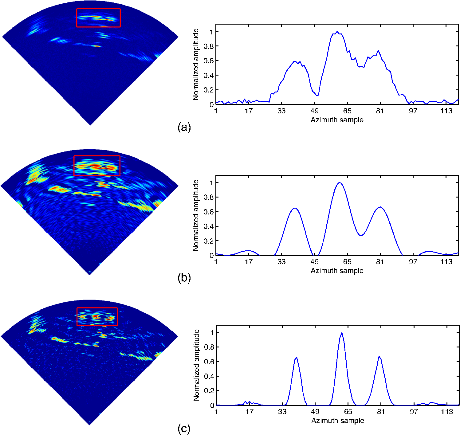

5.

Conclusion

This paper presents a deconvolution algorithm for angular super-resolution in scanning radar. After presenting and analyzing the signal model of the scanning radar, we first convert the angular super-resolution problem into an equivalent deconvolution problem. In order to overcome the ill-posed nature of the deconvolution problem, the deconvolution problem is converted into a constrained optimization problem by incorporating the prior information about the targets. Finally, the constrained optimization problem is solved in the framework of the augmented Lagrangian method. Compared with the conventional Wiener filter method, the presented deconvolution algorithm improves the angular super-resolution performance of the scanning radar in terms of precision. Simulations and experimental results show a better performance of the presented method compared with the traditional Wiener filter method. However, there are still some issues that need to be studied in angular super-resolution based on the deconvolution method. Future work will study the robustness of the deconvolution algorithm for angular super-resolution under low SNR levels.