1.

Introduction

Rice is the majority food in Asia area, which is widely planted in China especially in Sichuan province (southwest China), where the paddies can be classified into various categories. Remote sensing of paddy with synthetic aperture radar (SAR) has been an important component in rice monitoring and yield prediction during the past decades. Microwave remote sensing has the merits of penetrating cloud cover, being suitable for all kinds of weather conditions, and available day and night. Thus, it is taken into account. The backscattering coefficient from satellite SAR systems is interpreted for rice growth monitoring. The SAR data, ERS-1/2,^1–2 JERS-1,³ RADARSAT-1/2,^4,5 and ENVISAT ASAR,^6,7 have been used to map and monitor rice growth in worldwide test areas. The temporal behavior was effectively reported in a number of studies based on these SAR data. Rice monitoring has been extensively researched in the world, especially in Asia, including in China;^8,9 there is much research in India,¹⁰ Japan,¹¹ and other southeast Asian countries.^12,13 Many well-known techniques, such as SAR inteferometry, SAR polarimetry, multiparametric SAR data, and so on, are used for plant parameter retrieval such as plant height, plant density, crop biomass, crop moisture, and two-way attenuation through the canopy.^14–17 Initial studies have shown that the backscattering coefficient of rice obtained with spaceborne and airborne sensors presents obvious temporal variations corresponding to the high growth rate of rice plants. This temporal change in rice growth stages is crucial to distinguish rice crops from other covering types. However, the aforementioned information is limited to certain incidence angles, partial polarization, and particular satellite images. A ground scatterometer has been used to measure and study the scattering characteristics of rice in different regions because of its full polarization responses of a paddy at different frequencies and various incidence angles.

Numerous experiments on paddy have been performed with ground-based scatterometers.^18–20 Comprehensive measurements were performed by Inoue et al.¹⁹ The data of the research consisted of daily microwave backscattering coefficients with five frequencies combination, full-polarization, and four incident angles for the entire rice crop period (from the first period before transplantation to the last period postharvest cultivation). The ground-based scatterometer experiments proved that the backscattering coefficient has a significant sensitivity to rice parameters, and has a strong correlation with height, density, leaf area index (LAI), and biomass of rice. A full polarization scatterometer was also used to accurately measure the backscattering coefficients of a flooded rice field at the L and C bands, and the incidence angles varied from 30 deg to 60 deg.²⁰

Although these ground-based scatterometers and satellite data were useful in assessing the sensitivity between the backscattering coefficient and rice growth, studies of simultaneous observation by using ground-based and space-based scatterometers during the rice-growing season are still seldom reported. Therefore, this paper is aimed at studying the biomass from rice paddies through the analyses of simultaneous ground-based scatterometer and ASAR observations. A biomass inversion algorithm based on a semi-empirical scattering model is used.

Incidentally, the characteristic rice parameter is analyzed with the backscattering coefficients. Several experiments are conducted to measure the radar backscatter of rice at the C-band and full polarization (HH, VV, HV, and VH) with angular response during its growth period. The $R$-square $F$ statistics and significance of the regression analysis are the basis of modeling and inversion.

2.

Measurement and Data

The test site (103°32′24″E, 30°24′11″N) is one of the experimental fields of the University of Electronic Science and Technology of China (UESTC), which is located in Qionglai County, Chengdu, Sichuan, China. During the rice growth period, scattering measurement data and ASAR data are acquired from the ground-based radar scatterometer (GBRS) and ENVISAT satellite, respectively. This section introduces the ground experiments and ASAR data parameters.

2.1.

Ground Experiments

The sensor of the GBRS is a frequency-modulated continuous-wave full polarization radar, and it is also a dual-antennae system that maintains monostatic radar performances.²¹ The system is equipped at the C-band (center frequency 5.3 GHz) with a pair parabolic antenna. In addition, the GBRS system has a tilt and its azimuth scanning capability depends on a special platform device, which can transfer the incidence angles or pitch angle range from 0 deg to 90 deg, and azimuth angles range from 0 deg to 360 deg, respectively. The incidence of the antenna can range from 0 deg to 90 deg automatically with different steps. Furthermore, it can measure the backscattering coefficient of regional targets at different angles. The rotation in azimuth allows the antenna to acquire more independent samplings at the same place.

The support platform is a hydraulic lift. The scatterometer was elevated to 12.5 m throughout the measurement period.

Polarimetric calibration of the scatterometer system was realized with the single-target calibration technique, which was achieved by measuring the backscatter cross section of a conducting sphere (diameters with 469 and 580 mm).²²

The paddy had been flooded since seeding until harvest.

The rice seeds were sown in a nursery on May 5, 2010. Then, the rice seedlings were transplanted in the measurement site on May 28, 2010 with a transplanting machine. The measurements were taken from June 11, 2010 to September 12, 2010, as the rice was harvested on September 14, 2010. The entire period was usually divided into eight growth stages (seedling, tillering, jointing, booting, heading, flowering, milk, and ripening stage). The eight stages of the rice growth as well as the harvest are shown in Fig. 1. Measurements in this paper were taken during the eight stages, as shown in Figs. 1(a) to 1(h), while Fig. 1(i) was photographed when the rice had been harvested.

Fig. 1

Photograph of rice growth stages season at radar measurement dates: (a) seeding (06/11), (b) tillering (06/25), (c) jointing (07/09), (d) booting (07/23), (e) heading (08/08), (f) anthesis (08/20), (g) milking (09/04), (h) ripening (09/12), (i) regenation (09/16).

The ground measured data of the paddy were also collected during the rice growth cycle. The research collected rice canopy height, rice biomass (fresh and dry weight of rice per square meter, $\mathrm{g}/{\mathrm{m}}^2$), LAI, canopy structure, or geometric description. The main parameters at the eight stages are listed in Table 1.

Table 1

Rice growth stages at radar measurement dates and the main parameters.

Date	Days after transplanting	Canopy high (cm)	Biomass (kg/m2)	LAI	Stem density (m−2)	Rice moisture (%)
June 13	13	36.1	0.269	0.55	57	83.6
June 25	25	70.7	1.159	2.24	189	85.1
July 10	40	88.9	2.560	3.50	196	82.7
July 23	53	110.6	4.218	4.63	184	85.6
August 8	69	132.1	5.384	5.27	196	74.5
August 20	81	126.6	5.960	5.28	170	76.0
September 5	97	138.9	5.865	4.28	172	75.5
September 12	104	138.9	5.486	3.55	170	74.4

In each experiment, we randomly selected at least 20 sampling points in the paddy field. Parameters in Table 1 include rice canopy height, biomass, LAI and stem density, and rice moisture. After harvest stage, sampling biomass was $3.56\mathrm{kg}/{\mathrm{m}}^2$, which mainly consisted of rice straw residues and ratoon.

2.2.

ASAR Data

Three scenes of ASAR images covering the entire study area were acquired (see Table 2) at the same time, which have a nominal spatial resolution of 30 m and a pixel size of $12.5\times 12.5\mathrm{m}$. The date of the ASAR data acquisition was June 18, and September 20 and 28, 2010, which were at the rice growth cycle. The imaging modes are IS3, IS4, and IS5, and their incidence angles ranging are 26.0 deg–31.4 deg, 31.0 deg–36.3 deg, and 35.8 deg–39.4 deg, respectively. Dates shown in Table 2 correspond to seedling stage (tillering stage), ripening stage, and postharvest stage. The three images were obtained 18, 112, and 120 days after transplanting, respectively, covering the five major periods of the rice growth cycle.

Table 2

Three advanced synthetic aperture radar (ASAR) images over the rice test site.

Date	Operating mode	Swath (θ deg), the incident angle of test site	Polarization	Calibration factor (K)
June 18	AP	IS3(26.0–31.4), 31.2 deg	HH/VV	965500
September 20	AP	IS4(31.0–36.3), 34.5 deg	HH/VV	1613500
September 28	AP	IS5(35.8–39.4), 39.2 deg	HH/VV	2515625

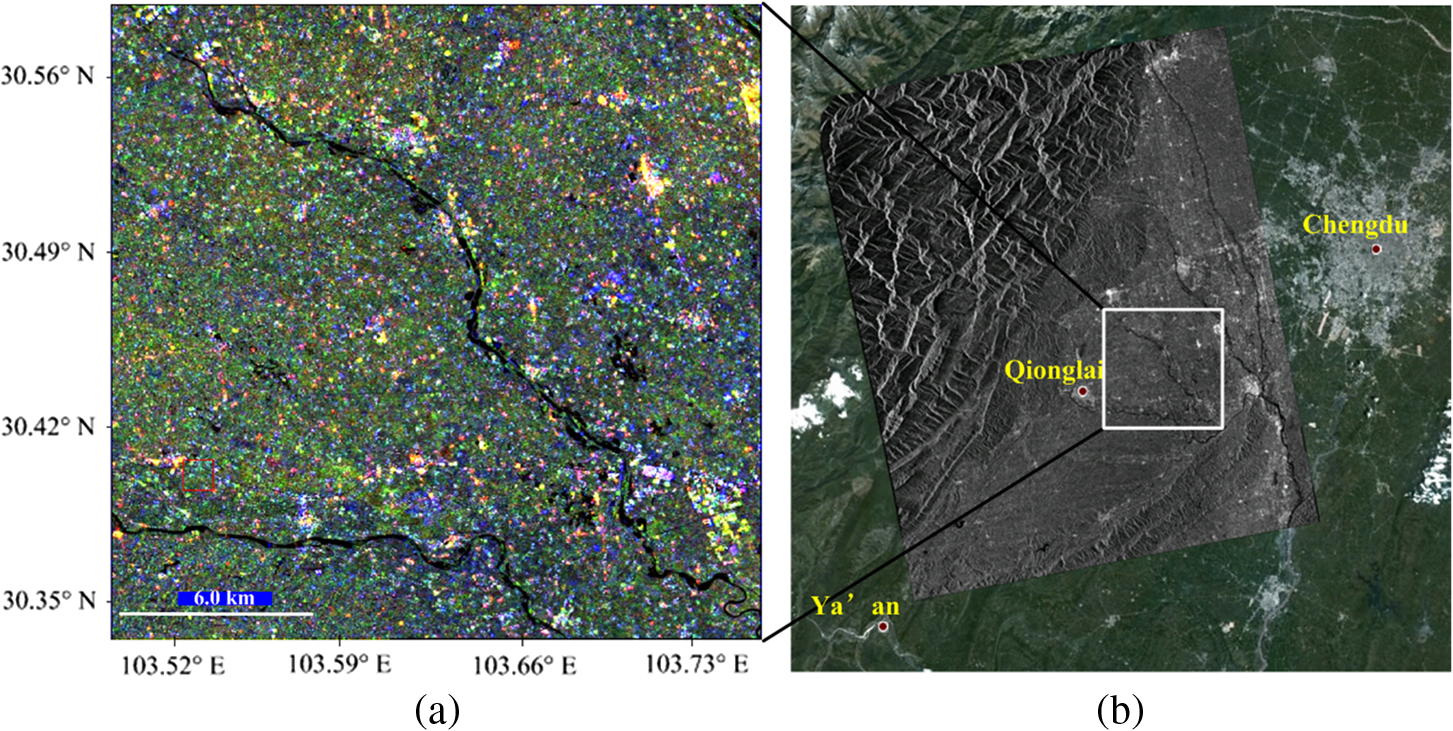
The Next European Space Agency (ESA) SAR Toolbox (NEST) was used in image preprocessing, which included radiance calibration, geocorrection, coregistration, speckle reduction, and data export. For geocorrection, the geographic Lat/Lon WGS84 was chosen as the coordinate reference system to reproject each SAR image. For the image coregistration, the number of ground control points is set to 200, and the root-mean square (RMS) threshold of pixel accuracy was chosen as 0.6. For speckle reduction, the multitemporal speckle filter was adopted to reduce the effect of speckle, and the filter window size was set to $7\times 7$. The data export included GeoTIFF products and Google Earth KMZ data. Figure 2 shows the test site location and an ASAR image. The color map is synthesized by the multitemporal image (R = June 18, G = September 20, and B = September 28) of HH polarization ASAR at the test site. The right part of Fig. 2 is the KMZ data of the SAR image (HH polarization, June 11) covered on Google Earth. This study selected was approximately a $20\times 20\mathrm{km}$ image region to meet the ground experiments. The test rice field (ground scattering measurement area) is marked with the red box area on the left part of Fig. 2.

Fig. 2

Test site location and advanced synthetic aperture radar (ASAR) image: (a) the multitemporal color composite image (R = June 18, G = September 20, and B = September 28) by using multitemporal HH polarization data, and (b) KMZ data of HH polarization SAR image covered on Google Earth.

3.

Data Analysis

The research successfully collected a wide range of data measurements and information during the entire rice growth season in 2010. All the measured data included the full polarization and the incidence angles from 0 deg to 80 deg. In order to show the backscatter characteristics of rice, all measured data of eight stages are illustrated in Fig. 3 as a function of the incidence angle. The temporal variations of full polarization at four selected incidence angles (25 deg, 35 deg, 45 deg, and 55 deg) have been analyzed with the rice grown stage in Fig. 4. Here, the polarization discrimination ratio (PDR) is selected as follows²³:

Fig. 3

Fully polarimetric backscatter values versus incidence angles for data referring to each measurement, (a), (b) (c), (d), (e), (f), (g), and (h) representing eight measured data values.

Fig. 4

Multitemporal backscatter values acquired of HH, VV, cross polarizations, and PDR and at (a) 25 deg, (b) 35 deg, (c) 45 deg, and (d) 55 deg incidence angles.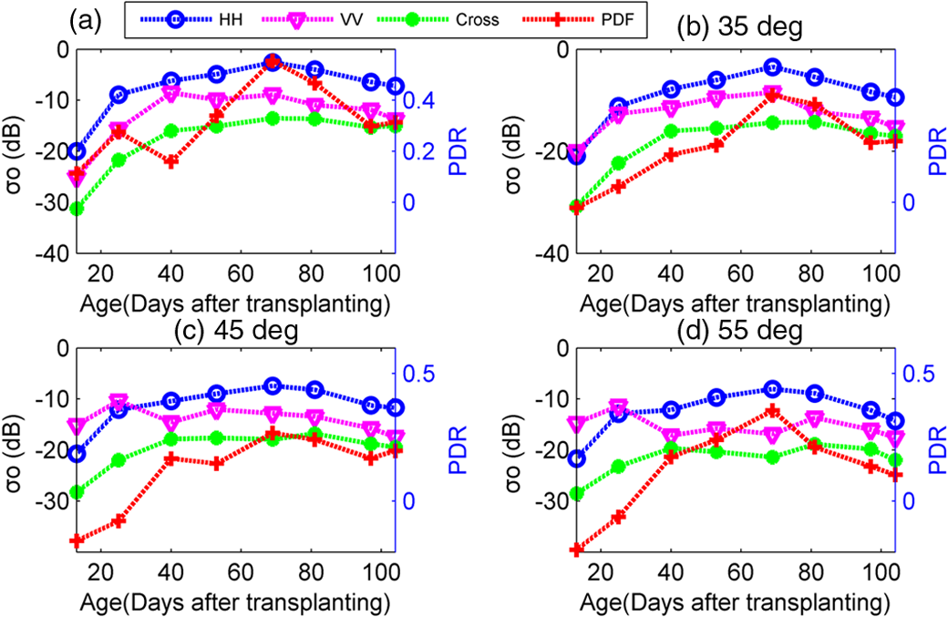

As shown in Fig. 3, the backscattering coefficients gradually decreased with the increase of incidence angles. However, the trends of the backscattering coefficients vary at different stages.

According to the different trends, the incidence angles can be divided into three ranges, including 0 deg to 20 deg, 20 deg to 60 deg, and 60 deg to 80 deg. In the first range, the backscatter coefficients decrease approximately in an exponential manner, which shows that the dominant scattering is reflected by the water surface directly. Thus, the reflection value is much greater than that reflected by canopy. The backscattering coefficient has a maximal value at 0 deg, but it rapidly decreases as the incidence angle increases. Furthermore, the peak value decreases with the growth of rice. As illustrated in Fig. 3, it was 12 dB in the first stage, whereas it dropped to about 5 dB in the fourth stage. It finally fell down to about $-8\mathrm{dB}$ in the last stage. This indicates that canopy attenuation increases significantly with the growth of rice. In stages of (c), (f), (g), and (h) shown in Fig. 3, the paddy is dry. Therefore, the scattering was contributed by soil, which is smaller than that by water at 0 deg incidence angle. Therefore, the scattering from the underlying surface continues to decrease.

At the second range, the decrease of the backscattering coefficient is approximately logarithmic because the scattering from the canopy is not sensitive to the incidence angle, and the dominant scattering changes to canopy scattering. In Figs. 3(c)–3(h), the backscattering coefficient of HH polarization is about 3–5 dB higher than that of VV polarization. Due to the vertical structure of the rice plant stems, the canopy scattering of HH polarization is larger than that of VV polarization, and the VV attenuation is higher than HH. Thus, the impact of the underlying surface (water or soil) on the total backscatter at VV polarization is significantly lower than that at HH polarization. The cross-polarized backscatter is similar to the HH polarization. However, the backscatter value of cross-polarization is about 8–10 dB smaller than HH polarization.

At the third range, the scattering for HH polarization continues to decrease, while VV polarization keeps constant or increasing, and the difference between HH and VV polarizations becomes smaller.

It implies that the vertical structure is not sensitive to polarization.

In particular, in Figs. 3(f)–3(h), the difference between HH and VV polarizations becomes smaller from 40 deg to 80 deg. This is probably because the emergence of the panicle undermines the vertical structure of the rice stem.

It can be seen from Fig. 4 that the backscattering coefficient is sensitive to the span since transplanting. The backscatter reaches a peak value 70 days after transplanting, which tends to decline slowly afterward. Therefore, the growing season of rice since transplanting can be divided into two separate periods. The first period (Age 0–70) started from the seedling stage to heading stage; and the second period (Age 70–104) from the flowering to ripening stage. During the first period, there is a very large change for each polarization. The range of HH polarization is larger than that of VV polarization. The maximum difference range of the backscattering coefficients is more than 10 dB between HH polarization and cross polarization at each incidence angle. This indicates that the temporal changes in the backscattering coefficients were more dynamic at small incident angles than at large angles. Moreover, the backscattering coefficient reaches the saturation point in the first period, but the scattering for VV polarization reaches saturation more quickly, with its saturation point at the jointing or booting stage.

In the second period, the backscattering coefficient shows a negative response to the rice changes, which declines about 3 dB at the end of the season. In addition, the largest difference between HH and VV polarizations appears during the rice booting stage, which is over 6 dB. However, the difference dropped to about 3 dB 40 days later. In short, the temporal change of the backscattering coefficient agrees well with the temporal change obtained for rice growth parameters in the first period. In comparison, the difference between HH and VV polarizations is distinctive for the rice paddy fields in the second period. Therefore, in order to effectively estimate rice-planted areas and monitor rice growth, using multitemporal observations for the first period is that the average of the temporal changes of the backscattering coefficient is more than 12 dB. In the second period, it is preferred to use multipolarization observations, since the average is over 5 dB. Table 3 shows the $r$-squared values between the polarization vector (HH, VV, Cross, and PDR) and the rice growth parameters (canopy high, biomass, LAI, stem density, and rice moisture).

Table 3

The r-squared value among backscatter of polarization vector (HH, VV, cross, and PDR) with the canopy high, biomass, leaf area index (LAI), stem density, and moisture of rice.

The $r$-squared statistic has been widely used in the literature to proxy for the quality of the information.²⁴ As shown in the table, the most accurate model is HH polarization with LAI ($r^2=0.92$), VV with stem density ($r^2=0.71$), cross polarization with LAI ($r^2=0.9$), and PDR with LAI ($r^2=088$), respectively. Rice biomass is highly correlated with the HH, cross, and PDR ($r^2=0.61$), while it is poorly correlated with the VV ($r^2=0.19$). LAI is strongly correlated with all of the rice growth parameters ($r^2>0.75$). Canopy height is also greatly correlated with the HH, cross, and PDR ($r^2>0.60$). Stem density is strongly correlated with HH, VV, and cross polarizations ($r^2>0.68$).

The $F$ test is used in the literature to measure the inversion accuracy. The inversed values $S_i$ and measured values $S_m$ are computed by the square of standard deviation equations into the $F$ test.²⁵ Then the $F$ value can be obtained.

The validation sample size $N_{\mathrm{validation}}$ is calculated in accordance with the literature:²⁶

These analyses show that multitemporal and multipolarization data have great potential in estimating rice-planted areas and monitoring rice growth.

4.

Inversion Model

The backscattering coefficient $\gamma$ for the whole canopy can be calculated with a simple process based on the semi-empirical water-cloud model (WCM),²⁷ which has been proven to be useful for a range of crop types and conditions.²⁸ The backscatter for the wheat field can be expressed as follows:

A flow chart of the inversion procedure is illustrated in Fig. 5. In the flow chart, all data are represented by a parallelogram. Input and output are distinguished by yellow and green, respectively. The inversion algorithm is marked with a light purple rectangular shape, and the image processing are marked with a gray rectangular shape. There are two types of data backscattering coefficients and multitemporal SAR images are used in the inversion process. The backscattering coefficients are measured and collected with a ground-based scatterometer. The multitemporal SAR images are obtained from ASAR (see Sec. 2).

Fig. 5

Main procedures of rice biomass retrieval using the experience model from the ASAR image.

The whole procedure can be divided into three parts. The left part is measuring and modeling. The right part is image processing and classification. In the middle, it is the inversion of the rice biomass. There are two steps to retrieve rice biomass. First, the inversion model should be established based on WCM with the measured backscattering coefficients, and the inversion results can be calculated from the SAR image. Second, apply the backscatter coefficients to the inversion model, which are extracted from SAR. Then, the output is the rice biomass maps.

5.

Results

The backscattering coefficients measured from ground scattering experiments are used for the model regression analysis. Since the model is nonlinear, the nonlinear least-squares estimation is used to estimate the coefficients of the WCM. In Fig. 6, the measured backscattering coefficients versus rice age are compared with modeled ones. Figure 6(a) is at HH polarization, while Fig. 6(b) is at VV polarization. The RMS errors $e$ and the coefficient of determination $R^2$ are marked on the graph. The RMS errors are 2.01 and 0.79 dB for HH and VV, respectively. And the coefficients of determination are 0.71 and 0.88, respectively. It can be seen from Fig. 6 that the modeled data from WCM accord well with the measured data. Table 4 gives the WCM coefficients of Eq. (7) at different incidence angles.

Fig. 6

Measured and modeled backscattering coefficients versus rice age at the C-band and 34.5 deg incidence angle: (a) HH polarization and (b) VV polarization.

Table 4

The WCM coefficients of Eq. (7) at different incidence angles.

In our paper, the RMS error is $1.05\mathrm{kg}/{\mathrm{m}}^2$, and the correlation coefficient is more than 0.86. Both values of biomass ($\mathrm{kg}/{\mathrm{m}}^2$) are obtained from Table 1 and Fig. 7. The degree of freedom and the average value are obtained easily as 7 and 3.86. Then, the $S_{\mathrm{m}}$ and $S_{\mathrm{i}}$ are calculated as 5.06 and 3.83, respectively, according to Eqs. (2) and (3). $F$ is 1.32 based on Eq. (4), where the confidence level is 95%. The $F$ test standard unilateral $F$ standard is 3.79. Obviously, the $F$ is smaller than $F$ standard. Therefore, the inversed values $S_i$ and measured values $S_m$ do not have statistical significance.

Fig. 7

Multitemporal trends of rice biomass: measured over the experimental site and simulations of the inversion model.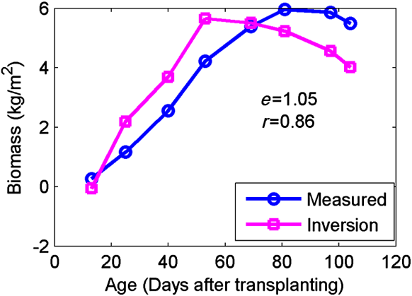

$N_{\mathrm{validation}}$ is given as 24. Thus, the validation sample size required for different cases can be computed using Eq. (5). Thus, one can determine the tentative validation sample size in advance based upon the expected $r_m^2$ value of model development sample. It shows that the trend of the biomass value is in accordance with the observed value. Thus, it can be concluded that the inversion model is valid.

After the estimation of the backscatter model, the biomass can be solved from Eq. (8) through optimization. Figure 7 shows the multitemporal trends of rice biomass, measured over the experimental site and simulations of inversion model. The RMS error is $1.05\mathrm{kg}/{\mathrm{m}}^2$, and the coefficient of determination is more than 0.86. It shows that the trend of the biomass value is in accordance with the observed value. Thus, it can be concluded that the inversion model is valid.

The backscattering coefficients of multitemporal ASAR images are extracted in the selected rice area. The area covers the ground experiment paddy site. Figure 8 shows the backscattering coefficients of paddy extracted from HH polarization images. Figures 8(a), (b), and (c) were obtained on June 18, and September 20 and September 28, respectively. Figure 8(d) illustrates the comparison of the backscattering coefficients using histograms.

Fig. 8

The extracted backscattering coefficients of test area from ASAR HH polarization images: (a) June 18, (b) September 20, (c) September 28, and (d) histograms of the backscattering coefficients.

As can be seen from the color bar, the light blue areas occupied the majority of the map. This implies the rice fields have low backscattering coefficients. The backscattering coefficient value of HH polarization mainly focused on the range of $-8.3\pm 2\mathrm{dB}$, $-6.5\pm 2\mathrm{dB}$, and $-6.3\pm 2\mathrm{dB}$ for June 18, September 20, and September 28, respectively. The mean value on June 18 is small, because the biomass is very small in the rice early growth stage. Thus, the backscattering is mainly contributed by the rice canopy and water surface. However, the biomass is large in the harvest period make the average values on September 20 and September 28 approach one another, both of which are larger than that on June 18. Thus, the backscattering is mainly contributed by the rice canopy and soil surface.

The backscattering coefficients of HH and VV polarizations that extracted from the ASAR image are used as the input parameters for the inversion model. Then, the biomass maps are outputted at three different periods. Figure 9 displays the results of rice biomass at different periods according to three ASAR images. As can be seen from the color bar and the histograms, the biomass maps show the distribution of the value of the biomass in a reasonable range for each image. Comparing different maps, it demonstrates the values of biomass differ in each growth period. As shown Fig. 9(d), the main values are in the range of about $1.2-1.6\mathrm{kg}/{\mathrm{m}}^2$, $3.5-5.5\mathrm{kg}/{\mathrm{m}}^2$, and $3.0-5.0\mathrm{kg}/{\mathrm{m}}^2$ for the three maps, respectively.

Fig. 9

Results of rice biomass in the test site at different periods from three ASAR images: (a) June 18, (b) September 20, (c) September 28, and (d) histograms of rice biomass.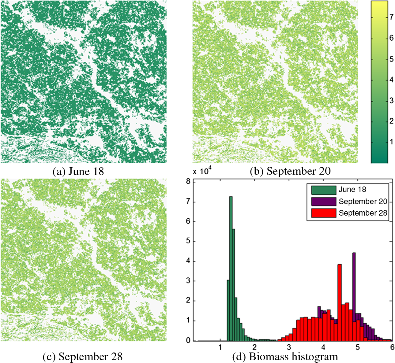

The corresponding values correspond to June 18, September 20, and September 28 are $1.159\mathrm{kg}/{\mathrm{m}}^2$, $5.486\mathrm{kg}/{\mathrm{m}}^2$, and $3.56\mathrm{kg}/{\mathrm{m}}^2$, respectively. In Fig. 9(a), most of the rice is at tillering and jointing stages (see Table 2), and the inverted average value was $1.246\mathrm{kg}/{\mathrm{m}}^3$, so the main color is dark green. In Fig. 9(b), the rice was mainly at the ripening stage and little rice has been harvested. The inverted average value was $5.206\mathrm{kg}/{\mathrm{m}}^3$, and the main color is yellow. The biomass is depicted as some small green areas, since rice has been harvested at this time. In Fig. 9(c), the inverted average value was $4.260\mathrm{kg}/{\mathrm{m}}^3$ and the main color is also yellow. However, the size of green areas is larger than that in (b), because more rice has been harvested in Fig. 9(c) compared with Fig. 9(b). Figure 10 shows the comparison of the retrieved biomass and measured biomass value in the test site at three growing stages. Most of the inverted results agree well with the measured values. The RMS error is $0.40\mathrm{kg}/{\mathrm{m}}^2$, and the coefficient of determination is 0.93. The results show that the proposed method using semi-empirical WCM performs well for these data. Therefore, multitemporal ASAR AP images can be used to monitor the growth of rice.

Fig. 10

Comparison of inverted and measured biomass of rice plants at three periods.

The inversion results are consistent with the actual growth of the rice area at each period.

6.

Conclusion

The paper investigates the radar sensitivity to rice biomass at the C-band with full polarizations in different rice phonological stages, and the process of the experiment was designed and described. A rice biomass inversion model was established based on the semi-empirical WCM by using measured data, and it was used to retrieve rice biomass from multitemporal ASAR AP images.

During the rice grown cycle in 2010, the measurement was carried out at the C-band with full polarization at 0 deg to 80 deg incident angles in eight successive rice growing stages. The ground data of the paddy field were also collected during the rice growth cycle at the same time, including rice canopy height, rice biomass, LAI, stem density, and rice moisture. The full polarization backscatter was analyzed as a function with the incidence angles at each rice growth period. The temporal variations of full polarization and PDR at four selected incidence angles (25 deg, 35 deg, 45 deg, and 55 deg) have been analyzed with the rice age. In the middle and late ages of the rice growth cycle, the backscattering coefficient for HH polarization is about 3–5 dB higher than that of VV polarization at a wide range of incidence angles (20 deg to 60 deg). In the entire rice growth cycle, the maximal range of HH backscattering coefficient is 10 dB more than those of cross polarizations at 25 deg and 35 deg incidence angles. The range of the backscattering coefficients at HH polarization is larger than that of VV polarization. The measured data show that it is better to use multitemporal data in the early rice growth and copolarimetric data in the late rice growth.

In addition, the coefficient of determinations between polarization vector (HH, VV, cross, and PDR) and the rice growth parameters (canopy high, biomass, LAI, stem density, and rice moisture) was calculated in the growth season. The results showed that the rice biomass is highly correlated with the HH and PDR.

An inversion model was established based on WCM by using the measured backscattering coefficients, and then the model was applied to invert rice biomass from the ASAR image. First, the measured backscattering coefficients under HH and VV polarizations were used to estimate the coefficients of WCM. The results showed that the simulated data from WCM agree well with the data measured.

Then biomass was obtained from the estimated WCM optimization after inputting the measured backscatter coefficients. The comparison of the measured data and estimated data based on the inversion model has proven the validity of the inversion model. Finally, the backscattering coefficients obtained from the multitemporal ASAR images in the selected rice area were used as the input of the inversion model, and the rice biomass maps were used as the output. Most of the inverted results are consistent with the measured values well at each period. The inversion results were effective because the RMS error is $0.40\mathrm{kg}/{\mathrm{m}}^2$ and the coefficient of determination is 0.93. The results showed that a good retrieval performance was obtained from these data by using the semi-empirical WCM.

In summary, the data analysis detailed and inversion applications show that multitemporal observation data at the early stage of rice growth and multipolarization observation data at the mid and late rice growth can be effectively used to estimate rice-planted areas and monitor rice growth. The inversion results show that the semi-empirical inversion model based on multitemporal SAR images at the C-band can be used to monitor the growth of rice.