|
|
1.IntroductionThe advent of high-resolution satellite images has increased possibilities for generating higher-accuracy land use and land cover (LULC) maps.1 Considering that urban classes are presented as a set of adjacent pixels, an object-based classification technique has an advantage over traditional pixel-based classification.2,3 These procedures utilize the spectral, geometrical, textural, and conceptual features of an image.4 As land use information cannot be derived directly from spectral information, an intermediate step of land cover classification is required.3 Many researchers have employed object-based methods to classify LULC from high-resolution satellite images.5–12 Most of these studies have been implemented in areas that are not complex or where a limited number of urban classes are available. Other researchers have applied textural and spectral information in an object-based analysis.13,14 These methods are mostly applicable to semiurban areas and can only detect a limited number of classes. To improve classification accuracy in urban areas, some researchers have integrated high-resolution and hyperspectral satellite images.15 Despite achieving acceptable accuracy, the necessity of having access to hyperspectral images is a major limitation of this method. Apart from the aforementioned considerations, the use of ancillary data, such as statistical and population information, for urban classification has been reported in other studies.9,16,17 Unlike land cover classification, fewer research works have focused on land use classification of land cover elements only based on the high-resolution satellite imagery in urban areas.3 In between them, even fewer have taken into account conceptual and spatial relations between land cover elements for land use classification. Differences in urban structure, local and cultural parameters, and development factors make it difficult to generalize land use classification model applications. Researchers believe that before land use information is extracted, spatial units of land use information must be determined.3,18 Various approaches have been used for the extraction of such land use spatial units (spatial extent of land use units). Studies have used manual drawings19 or ancillary data, such as road network maps,18 at the same time. Other researchers have used land cover information for extracting land use spatial units. Clustering criteria of building class as a basic element in urban areas are used for this purpose.18 This approach needs accurate extraction of building elements using ancillary data, such as LiDAR. In other approaches, linear elements, such as roads and linear vegetation features, have been used.3 Uncertainties are an obvious part of land use extraction. Low accuracy in dense urban areas is the most common problem using the aforementioned methods, which usually have been implemented in well-structured urban areas and are not practical in developing countries.18 Moreover, these approaches are efficient in extracting land use information over large regions (coarser spatial resolution) rather than detailed information at the land cover object level (finer spatial resolution). Additionally, errors from land cover classification can propagate and influence the extraction and classification of land use elements. The other main issue in land use analysis is in the classification stage. The simplest automated land use classification methods directly assign one or more land cover types to land use classes. This approach requires additional data across time. Moreover, a land cover class may be placed in multiple land use classes or vice versa. A more sophisticated approach uses a moving window or a kernel over a land cover layer. In this method, neighboring and spatial relationships between land cover classes are informative.18,20,21 However, selection of the best kernel size and probable geometric mismatches of land use unit shapes with the rectangular shape of the kernel are the most important weaknesses of this method. A method based on predefined land cover information has been used by some researchers. This approach comprises a step-by-step cycle of segmentation and classification based on limited conceptual features, such as vegetation or building percent area.3 The classification order assignment in this approach is based on ease of extraction. Because of intricate relations between land use classes, this strategy cannot be used in all urban regions. In this paper, we propose two novel algorithms (one supervised and one unsupervised) to automatically generate LULC maps from multispectral remotely sensed images.22 This research proposes a hierarchical LULC classification based on image objects that are created from a multiresolution segmentation. A rule-based strategy is used to implement a step-by-step object-based land cover classification. The order of classification of each land cover class is based on the class separability. To improve the overall accuracy of the land cover classification, we also use a new spatial geometrical analysis for reclassifying unclassified land cover objects. After these stages, an object-based step-by-step land use classification was designed and implemented based on the land cover results and using conceptual, spatial, and geometrical modeling of relationships between land use elements. The order of classification of each land use class is based on the independence ability in the conceptual and spatial relationships between the land use classes. This work differs from previous research in that multistage classification is implemented using image segmentation as well as contextual and geometrical spatial information, within a hierarchy-based scheme. 2.MethodsThe major steps of this research consisted of the following: (1) land cover classification model design and implementation, (2) land cover unclassified objects analysis, and (3) land use classification model design and implementation. Figure 1 illustrates the research methodology of this paper. To implement the proposed approach, a pan-sharpened IKONOS image from a complex urban area and a digital surface model (DSM) of Shiraz, Iran, were used [Fig. 2(a)]. Shiraz is located in the southwest of Iran, and it is the sixth most populous city of Iran and the capital of Fars province. Figure 2 shows the selected input image, DSM, and its corresponding reference map. The DSM layer was generated from aerial stereo image pairs recorded by the National Cartographic Center of Iran. The resolution of the generated DSM was 0.5 m and the vertical accuracy was 1 m. The reference map, which was used for accuracy assessment, was provided by the National Cartographic Center of Iran at a scale of . In addition to the land cover information for validation of the land cover classification, the reference map has enough information for the land use categorization of each element. Fig. 2Case study: (a) area in Shiraz, (b) IKONOS image, (c) digital surface model, and (d) the reference map.  The city of Shiraz has a high density of buildings, narrow secondary roads, and high diversity in main roads and building classes. Vegetation in the form of trees and gardens and many cars on the roads make the classification of this area at high spatial resolutions quite complex. 2.1.Image SegmentationAny object-based analysis is based on image objects created from an image segmentation step. Multiresolution segmentation is a bottoms-up region-merging technique starting with 1-pixel objects. In numerous subsequent steps, smaller image objects are merged into larger ones. Throughout this pair-wise clustering process, the underlying optimization procedure minimizes the weighted heterogeneity of resulting image objects, where is the size of a segment and a heterogeneity parameter. In each step, that pair of adjacent image objects are merged, which results in the smallest growth of the defined heterogeneity. If the smallest growth exceeds the threshold defined by the scale parameter, the process stops. Heterogeneity in multiresolution segmentation initially considers object features such as color and shape [Eqs. (1) and (2)]. The parameters and in Eq. (1) represent weights and demonstrate the amount of effect of any of these factors in approximating parameter . The spectral heterogeneity [Eq. (3)] allows multivariant segmentation by adding a weight to the image channel . The spectral heterogeneity is defined as where (: merge, obj1 and obj2) is the number of pixels within the merged object, object 1 and object 2, and is the standard deviation within the object in channel c for those three objects. To estimate [Eq. (4)], it is essential to estimate [Eq. (6)] and [Eq. (7)] and their weights [Eq. (5)] as well. These represent divergences that are obtained from the compactness and smoothness of the object’s geometry. where is the perimeter of the object and the perimeter of the object’s bounding box. , , , , and are weight parameters that can be selected to obtain suitable segmentation results for a certain image data. By determining parameter , computed for the candidate integrated object, this criterion is compared with the segmentation threshold limit scale () and the object integration process will continue up to the end of the threshold limit scale. Object-based systems have the capability of creating various segmentation levels such that any object can be related with other objects in its sublevels or superlevels. For implementation of image segmentation, scale and the weight parameters for each level must be selected.In high-resolution images of an urban area with a variety of heterogeneities, the least weight for spectral heterogeneity must be selected; otherwise, unnatural geometrical shapes will be created for objects and geometrical features can be lost. In the lower scale levels, the variety of heterogeneities is smaller than higher scale levels, so the weight of spectral heterogeneity must be decreased with increasing scale levels. High values for the parameter will make objects with compact forms. Under these conditions, classification of image object classes with linear characteristics is laborious compared to nonlinear object classes. Based on the previous discussion and empirical analysis, for LULC classification, three segmentation levels were used. The parameters for these are shown in Table 1. Table 1Segmentation parameters of the three levels.
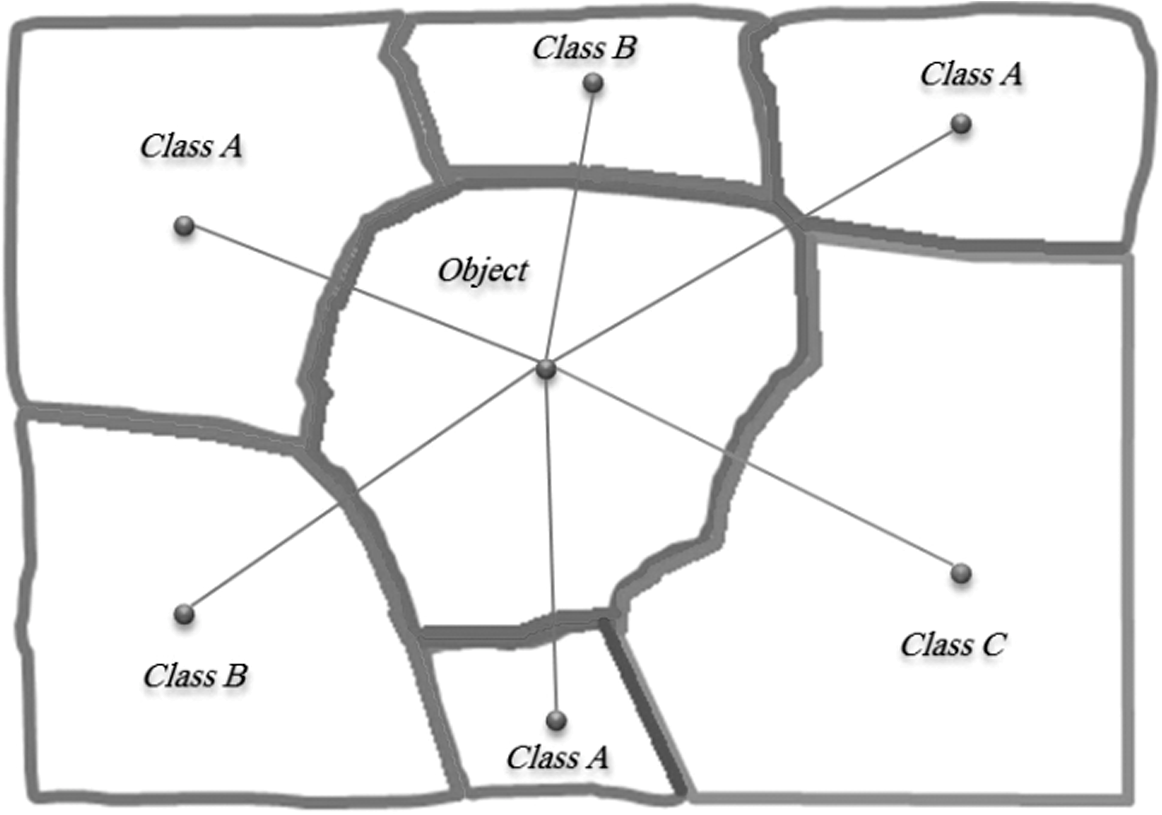
2.2.Land Cover Classification2.2.1.Rule-based land cover classificationConsidering the complexity of urban elements, it is necessary to design a stable strategy for land cover classification. The aim of the proposed rule-based land cover classification approach was to obtain least rules and feature space for the description of dense urban land cover classes. To achieve this, a step-by-step strategy was implemented (Fig. 3). In this method, the land cover classes were classified one after another and in a predetermined order. The main strategy in the design of this arrangement is based on higher separability and class significance. Given the spectral characteristics of vegetation classes in the visible bands, vegetation classes have the best conditions for classification and so were classified first. After classification of the vegetation class, its objects were reclassified into tree and grass classes. By merging tree neighbor objects, this class was reclassified into single tree and garden tree (cluster) classes. The building objects, using the features based on the DSM, were classified in the next stage. The buildings, based on the DSM features, were reclassified into one, two, or more than two story (level) classes. After these stages, the road classes (considering the class importance criterion) were detected. Road class objects were reclassified into main and secondary road classes. Considering the spatial and conceptual correlation between car and bus elements with roads, the objects of these two classes were classified in the next stage. The shadows have higher separability between the remaining classes. The bare soil and open space class with high spectral heterogeneity and any geometrical attributes were classified at the end. According to the significance measure, the road class was extracted after these two classes. Vehicle and shadow classes were classified in the next stage. The bare soil and open space class with its spectral diversities, which have the least geometrical and conceptual attribute, were classified in the final stage in this model. Fig. 4 shows the rules and feature space for classification of various land cover classes based on the rule-based model in Fig. 3. The rows in this table show the classes and the columns define the feature space used in the rule-based classification. In Fig. 4, the required features for the separation of mixed classes and the threshold for each feature are provided. It is important to mention that the logical relation between the class rules is AND logical operator. To separate the vegetation class, the Normalized Difference Vegetation Index (NDVI) was used. For uncertainty management created by the segmentation step, fuzzy thresholding on the NDVI was used. For this, a fuzzy s-shape membership function was designed for classification of the vegetation class. In fact, part of a plant may include nonvegetation pixels and vice versa, which shows fuzzy properties. Thus, in the vegetation and nonvegetation cluster center determination, fuzzy concepts must be considered. Accordingly, the fuzzy c-means clustering algorithm17 was used to locate the vegetation and nonvegetation cluster centers. Vegetation and nonvegetation object samples were collected from red and near-infrared (NIR) bands, and the NDVI image and the c-means algorithm for fuzzy clustering was performed for each pair. The results of this implementation are demonstrated in Fig. 5. Fig. 5Cluster centers: (a) NIR, red, (b) red, Normalized Difference Vegetation Index (NDVI), and (c) NDVI, NIR.  The NDVI cluster center was calculated from the centers of the red and NIR bands. The vegetation and nonvegetation cluster centers were calculated from the average of the preliminary NDVI clusters and the measured value of the NDVI cluster. Considering the obtained final NDVI amount for vegetation and nonvegetation classes, designing the s-shape function was thus completed. Figure 6 illustrates the s-shape designed membership function and the histogram of the NDVI data. Fig. 6NDVI histogram, designed membership form, and the amount of vegetation and nonvegetation cluster centers. Vegetation cluster center principal ; nonvegetation cluster center index .  According to Fig 4, the objects for which the fuzzy NDVI value is in level 30 were allocated to the vegetation class. After this, vegetation objects were merged using the merge region method. For tree and grass class separation from the vegetation class, mean brightness in all visible bands was used to highlight differences in density leaf and water capacity. Tree class objects have a high threshold for red, NIR, and green bands. The grass class has a low threshold for these bands. For this reason, the NDVI is not suitable for detection of these two classes. After this stage, a mask was made from vegetation classes and the other classes were classified in the nonvegetation part. The tree class objects were merged by a merge region algorithm. After this, the area feature was used for classification of garden tree and single tree classes. For classification of building subclasses based on number of levels, first the building objects were merged with the condition that the utmost value of the standard deviation of DSM for the merged object was . After this stage, the mean value DSM of the merged object was deduced from the minimum value of its neighboring objects. The value obtained showed the height value of the building object. Finally, the height value was divided by 3.3 m (the approximate height of a level), and the building objects were subclassified into three classes: one level, two levels, and more than two levels. 2.2.2.Unclassified land cover objects analysisAs a novel strategy in each step, some of the small objects were removed from the classification results based on the natural dimension of each desired urban class to obtain a smooth classification without any noise. Consequently, a final stage for the reclassification of these objects must be considered. Our strategy used the classification results of neighbors for the reclassification of unclassified objects. Based on logical relations between urban objects, the possibility of an unclassified object having the same class as one of its neighbors is quite high. Three geometrical/spatial features were designed and extracted for all of these objects. The first feature was the number of classified neighbor objects (NCNO) feature based on each class for unclassified objects. The second was the total common boundary (TCB) feature between the object and its neighbor objects based on each class. The third feature was the minimum distance between centers of gravity (MDCG) feature for the unclassified object and its neighbor objects. Unclassified objects were classified based on each one of these features. Figure 7 shows an example of the classification scheme. According to this example, the unclassified object is classified into class A based on the NCNO and TCB features, and class B based on the MDCG feature. In the TCB and NCNO features, unclassified objects are classified to a class that has a maximum value of this feature between the other classes for the desired unclassified object. However, in the MDCG feature, the desired unclassified object must be classified into a class with the lowest value. 2.3.Land Use ClassificationLand use classification generally cannot be derived directly from spectral or geometrical features based on satellite images. Therefore, extraction of land use information is conceivable based on land cover information. Land use classification was performed on level 3 and for four classes (road, building, vegetation, and bare soil-open space) that have a land use concept. 2.3.1.Step-by-step land use classification modelAs there are many relations between land use classes, a step-by-step land use classification model was designed accordingly and implemented in this study. This model commences with the land use classification of the road class, followed by land use classification of the building area. Vacant space and green space were classified in the next stages of this model (Fig. 8). The road land use class has the most independent attributes compared to the other land use classes, and based on the proposed model, the road class is considered the final step of land use classification. In this study, traffic measure was used for road land use classification. As a consequence, traffic criterion was the best feature to show the concentration of urban area activities in a satellite image. The remaining classes were then defined based on the relations and spatial arrangements of the land cover classes and the road land use classes. The order in the proposed land use model is based on class independency. Road land use classification.The simplest strategy for the classification of transportation land use regions is that all road objects in land cover levels are classified into the transportation class. However, in this research, we attempted to subclassify tranportation areas into a number of classes based on traffic measures. This measure is the only observable criterion of urban activity concentration in a satellite image. The road class is subclassified into two classes based on car and bus objects. The common border feature of the main road land cover class with vehicle classes is used for transportation land use classification. Before this stage, the main road class objects need to be preprocessed. Indeed, road objects must be analyzed with similar conditions. In using a common border feature, main road objects must have similar dimensions. The merge region approach for merging of the main road class was used. The condition that the merged object should not have a length was used. The main reason for the length feature in the merging condition is that the road class has generally linear attributes and vehicles run in the length direction of the road. By using this condition, the common border of the road class with the vehicle class is not an optimized feature. Actually, the dimension of the road merged objects influences this classification. So an index feature, the ratio of the aforementioned feature in the object area, was used. In addition, secondary roads were classified in the alley land use class (Fig. 8). Building land use classification.In developing countries such as Iran, the regional land use arrangement is generally based on local prospects. So, for example, institutional and commercial areas are comixed, and residental and commercial spaces are located adjacent to each other. Because of this heterogeneous form, the only way to recognize institutional-commercial regions is by utilizing the traffic in the margin of these regions during the daily crowded period. The margin building parts of urban blocks closer to the crowded main roads class are classified as institutional-commercial, and the inner regions of blocks are classified as residental. Before the implementation of this stage, building objects were merged with the condition that the area was (the approximate area of a building in the case study). For building land use classification, a class related conceptual feature was used. With this feature, the merged building objects that were placed at a distance from the crowded main roads class were classified as institutional-commercial building space. The building regions placed at a distance from the crowded main roads class and from the alley class was classified as residental. The remaining building objects that had common border with garden tree or grass classes were defined as recreational or green space building area (Fig. 8). The threshold value was determined based on experimental analysis. Vacant space land use classification.The concept of this class is contrary to land use concepts. The main purpose of the land use classification of vacant space was to meet planning requirements for the management of this region based on its proximity to other land use classes. All of the vacant areas have different planning costs. This class is either merged with residential and commercial regions or not classified at all in many studies. The bare soil-open space class was subclassified into three classes: commercial vacant, residential vacant, and green space vacant regions. The criteria for this classification included the distance from crowded main roads, commercial, residential, garden tree, and grass classes. Recreational and green space land use classification.A common green space in urban areas is the margin green space of the streets. For classification of this class, spatial and geometrical features were used. The spatial feature was the distance to the main road land cover class for all vegetation classes. This class has linear attributes similar to the road class. The next feature was length/width, which was used for the description of the linear classes. The next class was grass land, where the grass class objects in land cover classification were merged with the condition that the area was . Garden or tree planted classes were classified after the merging of garden tree class objects. The remaining green space classes were residential and commercial. The objects of these classes were classified based on their distance from commercial and residential regions. 3.Results and Discussion3.1.Land Cover Classification ResultsThe results of rule-based land cover classification are shown in Fig. 9. Fig. 9Results of land cover classification in various hierarchies. The second set of images shows the zoomed-in region marked in (c). (a) separating buildings class from nonbuildings, (b) classifying the nonbuildings class into vegetation, roads and open spaces, and (c) final level of classification of the buildings, vegetation and open space classes.  Based on the proposed unclassified analysis approach, 100 random unclassified objects were selected and then real classes for each random sample were determined using a reference map and visual interpretation. Table 2 shows the result of the unclassified objects analysis using the aforementioned features. Table 2Accuracy assessment of unclassified objects.
The accuracies obtained were calculated based on two criteria: with object area weight and without object area weight. Based on the previous table, the center of gravity feature has the best result. Based on this feature, of the unclassified objects were correctly classified. Accuracy assessment criteria for the land cover classification are shown in Table 3. Table 3Accuracy assessment of land cover classification.
Accuracy assessment was performed based on the object samples provided from the existing reference map. The overall accuracy and kappa were 89% and 0.86, respectively. Regarding the complexities of the case study, the accuracy obtained was satisfactory. The vegetation classes were classified with 95% accuracy. Grass and the two tree classes had mixed objects. The car and bus classes were classified with high accuracy (both ). These two classes have spectral and geometrical similarities with building classes, but by using the DSM layer and conceptual features in building classification and two vehicle classes, respectively, they had low mixed objects. Nonetheless, the user accuracy of the building class was . 3.2.Land Use Classification ResultsThe results of the land use classification are shown in Fig. 10. The comparison of reference data with the results of selected land use classes is shown in Fig. 11. Fig. 11Top row—reference map (commercial space sample, grass land space, garden space, main road). Bottom row—classification results (commercial space, grass land, garden space, highly crowded main road, less crowded main road).  The results demonstrate the effectiveness of the proposed land use classification model. The main road class in the reference map is classifed into two classes: highly crowded or less crowded. The proposed approach classifies these two classes based on instantaneous vision (as captured by the satellite image). Table 4 shows the accuracy assessment of land use classification. Table 4The accuracy assesment of land use classification results.
The overall accuracy was 86.8%. Based on the area weight for any land use class, the overall accuracy was 88.9%.The accuracy assesment of the results, with high detail and without any additional data, shows the effectiveness of the proposed approach. The vegetation class has low accuracy for two reasons. The width of some real vegetation objects were (e.g., shrubs) and, according to the resolution of the pan-sharpened IKONOS image, these objects could not be recognized. The time difference between the reference data and the IKONOS image capture also lowers accuracy. 4.ConclusionIn this research, an object-based method based on a hierarchical model for land use and land cover classification in a dense urban area from high spatial resolution satellite images is presented. We propose a contiguous cycle of approaches to extract land use information from high-resolution imagery. In the first step, a rule-based land cover classification was designed and applied using object-based features including spectral, geometrical, and conceptual. In the proposed method, a step-by-step strategy is used. Evaluation of results obtained from the implementation of the proposed approach on an IKONOS image from a dense urban area showed the efficiency of this method. The most important achievements of this research include satisfactory classification results in a complex dense urban area with no need for training samples. The class hierarchy of the proposed rule-based land cover classification includes 16 classes at two levels. Classes such as car and bus are used for finding the centers of activity in the land use classification for defining commercial and institutional regions. The main purpose of using this class hierarchy is to apply a stable and detailed input for land use classification analysis. The hierarchical order of the land cover classes is based on the classification capability of the classes and class significance. After the implementation of land cover classification, a geometrical spatial analysis is used for the reclassification of unclassified objects in the land cover stage. The distance between the gravity center feature gives the best result in the reclassification of unclassified objects. In the land use classification phase, a stage-by-stage strategy is used. In the present study, conceptual relations and attributes between land cover classes are used for the implemetation of land use classification. Attributes such as traffic reflect the concentration of activity in urban areas and are likely used for the first time in this study. The combination of methods proposed in this paper results in fewer unclassified objects since a multistage classification process is utilized rather than the traditional one-pass classification. Furthermore, the proposed approach emphasizes the use and modeling of conceptual knowledge and regional information as an appropriate tool to exploit the information content of high-resolution images in land cover and land use analysis. The methods described here result in a land use layer as well as a land cover layer, with objects as small as a car being classified with high accuracy due to the use of contextual as well as geometrical spatial information. ReferencesR. Zhang and D. Zhu,
“Study of land cover classification based on knowledge rules using high-resolution remote sensing images,”
Expert Syst. Appl., 38
(4), 3647
–3652
(2011). http://dx.doi.org/10.1016/j.eswa.2010.09.019 ESAPEH 0957-4174 Google Scholar
U. C. Benz et al.,
“Multi-resolution, object-oriented fuzzy analysis of remote sensing data for GIS-ready information,”
ISPRS J. Photogramm. Remote Sensing, 58
(3), 239
–258
(2004). http://dx.doi.org/10.1016/j.isprsjprs.2003.10.002 IRSEE9 0924-2716 Google Scholar
M. Lackner and T. M. Conway,
“Determining land-use information from land cover through an object-oriented classification of IKONOS imagery,”
Can. J. Remote Sens., 34
(2), 77
–92
(2008). http://dx.doi.org/10.5589/m08-016 CJRSDP 0703-8992 Google Scholar
J. Schiewe and M. Ehlers,
“A novel method for generating 3D city models from high resolution and multi‐sensor remote sensing data,”
Int. J. Remote Sens., 26
(4), 683
–698
(2005). http://dx.doi.org/10.1080/01431160512331316829 IJSEDK 0143-1161 Google Scholar
M. Herold et al.,
“Object-oriented mapping and analysis of urban land use/cover using IKONOS data,”
in 22nd Earsel Symp. on Geoinformation for European-Wide Integration,
4
–6
(2002). Google Scholar
L. Gusella et al.,
“Object-oriented image understanding and post-earthquake damage assessment for the 2003 Bam, Iran, earthquake,”
Earthq. Spectra, 21
(S1), 225
–238
(2005). http://dx.doi.org/10.1193/1.2098629 EASPEF 8755-2930 Google Scholar
R. Mathieu, C. Freeman and J. Aryal,
“Mapping private gardens in urban areas using object-oriented techniques and very high-resolution satellite imagery,”
Landsc. Urban Plan., 81
(3), 179
–192
(2007). http://dx.doi.org/10.1016/j.landurbplan.2006.11.009 LUPLEZ 0169-2046 Google Scholar
J. Inglada,
“Automatic recognition of man-made objects in high resolution optical remote sensing images by SVM classification of geometric image features,”
ISPRS J. Photogramm. Remote Sens., 62
(3), 236
–248
(2007). http://dx.doi.org/10.1016/j.isprsjprs.2007.05.011 IRSEE9 0924-2716 Google Scholar
Y. Chen et al.,
“Object‐oriented classification for urban land cover mapping with ASTER imagery,”
Int. J. Remote Sens., 28
(20), 4645
–4651
(2007). http://dx.doi.org/10.1080/01431160500444731 IJSEDK 0143-1161 Google Scholar
C. Cleve et al.,
“Classification of the wildland-urban interface: a comparison of pixel-and object-based classifications using high-resolution aerial photography,”
Comput., Environ. Urban Syst., 32
(4), 317
–326
(2008). http://dx.doi.org/10.1016/j.compenvurbsys.2007.10.001 CEUSD5 0198-9715 Google Scholar
G. Ruvimbo, P. De Maeyer and M. De Dapper,
“Object-oriented change detection for the city of Harare,”
Expert Syst. Appl., 36
(1), 571
–588
(2009). http://dx.doi.org/10.1016/j.eswa.2007.09.067 ESAPEH 0957-4174 Google Scholar
W. Zhou et al.,
“Object-based land cover classification of shaded areas in high spatial resolution imagery of urban areas: a comparison study,”
Remote Sens. Environ., 113
(8), 1769
–1777
(2009). http://dx.doi.org/10.1016/j.rse.2009.04.007 RSEEA7 0034-4257 Google Scholar
R. R. Colditz et al.,
“Influence of image fusion approaches on classification accuracy: a case study,”
Int. J. Remote Sens., 27
(15), 3311
–3335
(2006). http://dx.doi.org/10.1080/01431160600649254 IJSEDK 0143-1161 Google Scholar
X. Liu, K. Clarke and M. Herold,
“Population density and image texture,”
Photogramm. Eng. Remote Sens., 72
(2), 187
–196
(2006). http://dx.doi.org/10.14358/PERS.72.2.187 PGMEA9 0099-1112 Google Scholar
L. Zhang and X. Huang,
“Object-oriented subspace analysis for airborne hyperspectral remote sensing imagery,”
Neurocomputing, 73
(4), 927
–936
(2010). http://dx.doi.org/10.1016/j.neucom.2009.09.011 NRCGEO 0925-2312 Google Scholar
J. Harvey,
“Estimating census district populations from satellite imagery: some approaches and limitations,”
Int. J. Remote Sens., 23
(10), 2071
–2095
(2002). http://dx.doi.org/10.1080/01431160110075901 IJSEDK 0143-1161 Google Scholar
K. Chen,
“An approach to linking remotely sensed data and areal census data,”
Int. J. Remote Sens., 23
(1), 37
–48
(2002). http://dx.doi.org/10.1080/01431160010014297 IJSEDK 0143-1161 Google Scholar
Q. Zhang and J. Wang,
“A rule-based urban land use inferring method for fine-resolution multispectral imagery,”
Can. J. Remote Sens., 29
(1), 1
–13
(2003). http://dx.doi.org/10.5589/m02-075 CJRSDP 0703-8992 Google Scholar
M. Herold, X. Liu and K. C. Clarke,
“Spatial metrics and image texture for mapping urban land use,”
Photogramm. Eng. Remote Sens., 69
(9), 991
–1001
(2003). http://dx.doi.org/10.14358/PERS.69.9.991 PGMEA9 0099-1112 Google Scholar
M. Barnsley and S. Barr,
“Inferring urban land use from satellite sensor images using kernel-based spatial reclassification,”
Photogramm. Eng. Remote Sens., 62
(8), 949
–958
(1996). PGMEA9 0099-1112 Google Scholar
D. Chen, D. A. Stow and P. Gong,
“Examining the effect of spatial resolution and texture window size on classification accuracy: an urban environment case,”
Int. J. Remote Sens., 25
(11), 2177
–2192
(2004). http://dx.doi.org/10.1080/01431160310001618464 IJSEDK 0143-1161 Google Scholar
A. Haldera, A. Ghosha and S. Ghoshb,
“Supervised and unsupervised land use map generation from remotely sensed images using ant based systems,”
Appl. Soft Comput., 11 5770
–5781
(2011). http://dx.doi.org/10.1016/j.asoc.2011.02.030 1568-4946 Google Scholar
BiographyMohsen Gholoobi is an MSc graduate in the field of remote sensing and has over seven years of experience. He received his MSc degree in remote sensing from Khaje Nasiredin Toosi University of Iran in 2011. He works in a research center related to remote sensing topics in urban and agriculture, target detection, and forest management. He has published 20 journal and conference papers. Lalit Kumar is an associate professor in ecosystem management at the University of New England in Australia. His expertise is in the fields of remote sensing and GIS technology related to natural resources management and agricultural systems. He has over 20 years of experience and has published more than 100 journal papers. He received his PhD degree in remote sensing from the University of New South Wales in Australia in 1998 and his MS degree from the University of the South Pacific in Fiji in 1992. |
||||||||||||||||||||||||||||||||||||||||||||||||||||||||||||||||||||||||||||||||||||||||||||||||||||||||