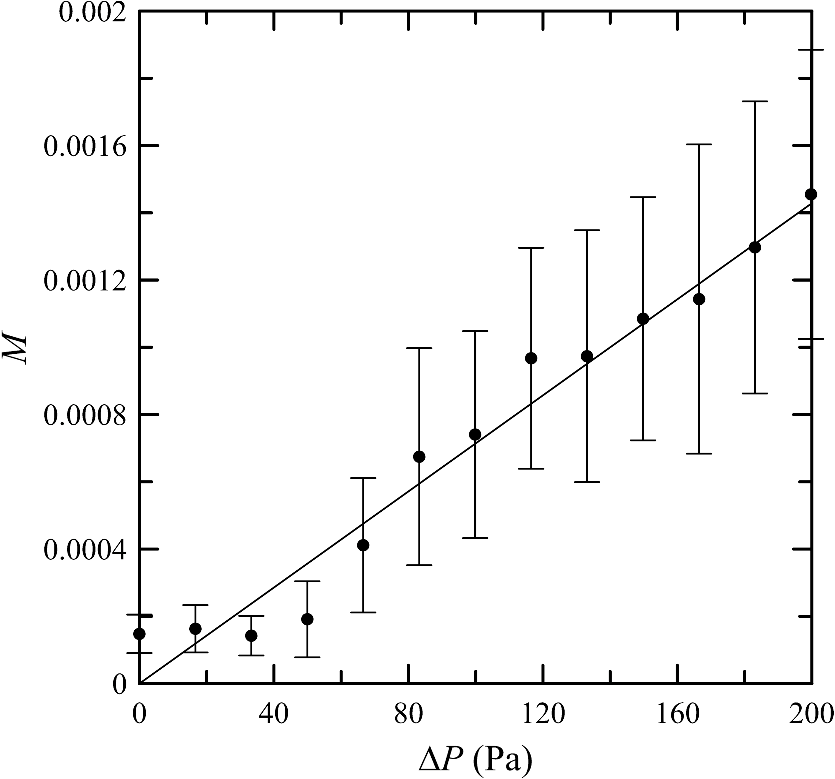
1.

Introduction

There are a number of reasons one might want to fly over the ocean and listen to the sound below the surface. Examples include measurement of shipping noise, tracking of marine mammals, and searching for the flight data recorder of a lost aircraft, like Malaysian Airlines flight MH370. Unfortunately, direct detection of sound from above is difficult because the transmission loss at the surface is 65 dB. The transmission loss at the surface for visible light is only $\sim 0.1\mathrm{dB}$, so a technique that uses visible light to interrogate the acoustic field just below the surface would be desirable.

Fabrikant suggested modulating a laser such that the wavelength of the modulation was Bragg-matched to the acoustic wavelength in water.¹ Small variations in the optical scattering induced by the acoustic wave would cause amplitude modulation of the scattered light. He showed how an acoustic wave moving toward the surface would produce a signal at the modulation frequency with a Doppler shift determined by the speed of sound.

Others have suggested using coherent optical detection of the light reflected from the sea surface to directly measure the motion of the surface induced by the acoustic pressure, and this technique has been demonstrated in laboratory tests.^2–4 The motion of the surface induced by the acoustic signal can be much smaller than the motion induced by surface winds, and separating the two effects using this technique can be difficult. One technique to accomplish this is to measure the statistical properties of the scattered laser light, which are affected by the acoustic signal.^5,6 This technique has also been demonstrated in a laboratory setting, but the application of this technique in the open ocean would be difficult.

This paper suggests another approach. Light scattered from bubbles that are always present near the ocean surface will be modulated at acoustic frequencies when the size of those bubbles is modulated by the pressure associated with the acoustic field. Airborne lidar can penetrate the air/sea interface into the near-surface layer of the ocean. This near-surface layer is where the bubble concentration is greatest.^7,8 Sound can propagate up from great depths to near the surface, so this technique has the potential to detect sound sources that are well below the penetration depth of an airborne lidar.

2.

Theoretical Background

If the frequency of sound is much less than the resonant frequency of a bubble, its relative volume will change adiabatically with a small change in pressure as

The resonance frequency is given by⁹

For a fixed frequency and a distribution of bubble sizes, bubbles that are at resonance and those not at resonance must be treated separately and the results added. Since $Q$ is the ratio of $f_0$ to the width of the resonance, a bubble will be in resonance for frequencies in the range

This implies that, for a frequency $f$, bubbles within the size range of

The lidar signal $S$ is proportional to the volume scattering function $\beta$ at the lidar scattering angle of $\pi$ radians. Using geometric optics, it is straightforward to show that the latter quantity is proportional to the void fraction $F_v$ of the bubbles within the lidar resolution element independent of the bubble size distribution.¹⁰ Neglecting possible resonance effects, the modulation depth of the lidar signal can be expressed as

Because the sound wave is almost totally reflected from the surface with a phase reversal, a standing wave is produced. The resulting acoustic pressure $\mathrm{\Delta }P(z)$ from an incident acoustic wave with wavenumber $k_a$ and amplitude $P_a$ is

The factor of two comes from the superposition of the incident and reflected acoustic wave. This has a maximum at a depth of $0.25{\lambda }_a$, where ${\lambda }_a$ is the acoustic wavelength. For a plane wave and flat surface, this same maximum value also occurs at $0.75{\lambda }_a$, $1.25{\lambda }_a$, and so on. However, this complete interference is not always observed in practice because of surface roughness, bubbles, and bottom reflections.^11,12

To be detectable, the modulation depth has to be greater than the relative fluctuations caused by noise processes. For a shot-noise-limited system, this implies that the minimum detectable sound pressure level is given by

3.

Experiment Description

These concepts were tested in a laboratory tank (Fig. 1) with a bubbler and speaker on the bottom and a laser source and optical receiver at the side of the clear glass tank. The tank itself is 60 cm wide by 180 cm long and was filled with water to a depth of 70 cm. The measurement volume was located 24 cm below the surface at a distance of 25 cm from one side of the tank.

Fig. 1

Schematic diagram of the tank experiment. A bubbler on the bottom is supplied with compressed air from a pump. A speaker is driven with a 5 kHz acoustic source. The laser beam illuminates the bubble plume from outside the tank, and a lens collects a portion of the scattered light onto a photodetector.

A plume of bubbles was produced by running compressed air through a ceramic filter (Sweetwater air diffuser model ALR150, 152 by 38 by 38 mm) with void fraction controlled by controlling the flow of air to the filter. This was oriented with the long axis vertical to produce a bubble plume that was nearly circular at the measurement volume with a diameter of 50 mm. This technique was chosen to get a relatively narrow bubble size distribution.¹³ For low void fraction, the actual size distribution and void fraction were measured using photographs of the bubble plume (Fig. 2). For each photograph, the contrast was enhanced, and then the area of each bubble was measured and converted to radius and volume.

Fig. 2

Example of contrast-enhanced bubble photograph used to measure void fraction and size distribution.

The average of the distributions from seven photographs (Fig. 3) shows a peak in the bin where $0.45\mathrm{mm}<a<0.5\mathrm{mm}$. The average radius was 0.61 mm and the rms width of the distribution was 0.20 mm. The void fraction was measured from those same images using the thickness of the plume, with a result of $(1.17\pm 0.12)\times {10}^{-3}$.

Fig. 3

Histogram of bubble radius, $a$. Error bars represent the standard deviation of values from the seven photographs.

At higher void fractions, the bubbles in the photographs could not be resolved, so another technique was used to estimate void fraction. The average bubble rise velocity was estimated from the smearing in a long-exposure photograph (20 ms), and the void fraction estimated from the bubble plume diameter, average bubble rise velocity, and the measured flow rate of air to the diffuser. Using this technique, the flow rate was adjusted to obtain a void fraction of 0.01.

A 5 kHz acoustic signal was generated digitally with 100 samples per cycle and an amplitude resolution of 16 bits. This was converted to an analog voltage, amplified, and sent to an underwater speaker suspended just above the bottom of the tank. The sound pressure was measured at the measurement volume with a hydrophone. Any effects of interference between the direct and reflected acoustic pressures are taken into account in this measurement.

The sound pressure levels were measured with an Aquarian Audio Products H1A hydrophone, which has a typical response of $-200\mathrm{dB}$ $\mathrm{re}1\mathrm{V}\mu {\mathrm{Pa}}^{-1}$ at 5 kHz. At low void fraction, the measured sound pressure level at the measurement position was linearly proportional to the drive voltage with a response of $1423\mathrm{Pa}{\mathrm{V}}^{-1}$. At higher void fraction, the sound pressure levels are reduced by attenuation by the bubble plume and are difficult to measure directly. To first order, this reduction should be proportional to the ratio of the void fractions for the two cases (a factor of 8.55), so the sound pressure at high void fraction was taken to be proportional to the drive voltage with a response of $166\mathrm{Pa}{\mathrm{V}}^{-1}$.

The optical source was a 40 mW stabilized laser operating at a wavelength of 532 nm. The beam was expanded to a diameter of 30 mm at the measurement volume with a diverging lens. The receiver used a lens to collect the scattered light onto a photodiode. The field of view of the receiver at the measurement volume was 31 mm. To reduce the amount of scattering from the tank, the receiver was offset at an angle of 16 deg from the transmitted beam.

The photodiode output was converted to a voltage with a transimpedance amplifier. The resulting voltage was sampled at 41 kHz by the 24-bit computer sound card to obtain the acoustic modulation. For each sound pressure, the power spectral density was calculated for 100 consecutive data segments that were each 1 s long (1 Hz spectral resolution). The same voltage was also sampled at 100 Hz by a dc coupled digitizer to obtain the average return. The modulation depth was calculated as

4.

Laboratory Results

A typical power spectral density of the optical signal (Fig. 4) shows a very narrow spectral peak at 5 kHz. $Q$ is 22.5 at this frequency. The sound pressure level, estimated using the manufacturer’s response, was 1700 Pa. SNR inferred from the plot is 57 dB.

Fig. 4

Example of the power spectral density function of the optical detector output as a function of frequency, $f$, for the low-void-fraction case.

For low void fraction, the measured modulation depth (Fig. 5) shows a clear increase in modulation depth with increasing sound pressure. The response is very nearly linear, except at the very lowest sound levels, where detector noise is an issue. One interesting feature of the three lowest points is the relatively small error bars; the variability of the detector noise on time scales of several seconds is much less than the variability in the bubble plume. From a linear regression, the slope of the response is $(1.08\pm 0.04)\times {10}^{-5}{\mathrm{Pa}}^{-1}$. The theoretical response in the figure, from Eq. (6), has a slope of $7.14\times {10}^{-6}{\mathrm{Pa}}^{-1}$. This difference is not within the statistical uncertainty of the regression, but is within the uncertainty in the hydrophone calibration ($\pm 4\mathrm{dB}$).

Fig. 5

Modulation depth, $M$, as a function of sound pressure amplitude, $\mathrm{\Delta }P$, for low-void fraction. Circles are averages of ten 1-s measurements, error bars represent the standard deviation of those measurements, and the solid line is the theoretical prediction.

For the higher void fraction, the measured modulation depth (Fig. 6) looks very similar, except that both sound pressure levels and modulation depths are roughly an order of magnitude lower as a result of the greater attenuation by the bubble plume. Here, the slope of the regression is $(7.14\pm 0.41)\times {10}^{-6}{\mathrm{Pa}}^{-1}$, and the close agreement with the theoretical value is largely coincidental. At this void fraction, more light is scattered by the bubble plume, so the signal to noise is greater and the modulation is visible above the noise at a lower sound pressure. The ratio of minimum detectable signals for the two cases is 6.4, or $\sim 75\%$ of the expected value based on the ratio of void fractions.

Fig. 6

Modulation depth, $M$, as a function of sound pressure amplitude, $\mathrm{\Delta }P$, for high-void fraction. Circles are averages of ten 1-s measurements, error bars represent the standard deviation of those measurements, and the solid line is the theoretical prediction.

5.

System Considerations

The lidar system needed to measure sound in the open ocean is different from existing systems, where the objective is to measure the vertical distribution of scattering particles like fish^14,15 and plankton¹⁶ in the water or to use the distribution of plankton to infer dynamical processes like internal waves.^17–19 Such systems require a high instantaneous dynamic range and often use polarization to enhance the return.^20,21 An acoustic detection lidar, on the other hand, does not benefit from the use of polarization, since the return from bubbles preserves polarization.¹⁰ A high dynamic range is not required, since the system only requires a single sample of the return from each transmitted pulse, at a constant depth, and this can be made near the surface. What is required is (1) a relatively high pulse-repetition rate in order to sample the return at acoustic frequencies and (2) a high SNR to measure the small modulation depths expected.

The SNR will generally be limited by shot noise in the photocurrent, which depends on the near-surface bubble void fraction.¹⁰ In bubble clouds associated with breaking waves, values between ${10}^{–4}$ and 0.01 have been observed.^22–24 The background void fraction is much lower. Thorpe et al.²⁵ reported values between ${10}^{–8}$ and ${10}^{–7}$ at depths of 2 to 4 m and winds near $10\mathrm{m}{\mathrm{s}}^{-1}$. Vagle et al.²⁶ present a probability distribution of measured values that shows most of the values between ${10}^{–8}$ and ${10}^{–6}$, with the most likely value just larger than ${10}^{–7}$. Gemmrich²⁷ measured void fraction at depths of 2.6 and 0.85 m between and within the convergence zone of Langmuir circulation. At the deeper location, the background void fraction was $<{10}^{-7}$, increasing to $>{10}^{-6}$ in the convergence. At the shallower location, the background was $\approx 5\times {10}^{-6}$, increasing to just under ${10}^{–4}$ in the convergence.

There are always some bubbles present, but most are produced by wind–wave interactions. An empirical model²⁸ predicts void fraction of

One difference between the laboratory experiment and a field system is that the latter must work through the sea surface. One consequence of this is that a fraction of the incident light will be blocked by whitecaps and foam, especially at high wind speeds. The fraction of the surface covered by whitecaps and foam can be estimated from the wind speed as $3.84\times {10}^{-6}{U}^{3.41}$.³² Less than 10% of the incident light will be blocked by whitecaps and foam unless the wind speed is $>20\mathrm{m}{\mathrm{s}}^{-1}$; winds this high are not common,³⁰ so this is not a serious limitation.

Another consequence of the surface is that waves can introduce fluctuations in the signal.³³ These could be important when there is a surface wave whose wavelength, $\lambda$, is equal to the ratio of the aircraft speed across the waves to the acoustic frequency of interest, or

The detection of blue whales (Balaenoptera musculus) in the Southern Ocean provides an example of system performance in the open ocean. These whales produce sound in a frequency band of 25 to 29 Hz with source strength of $189\pm 3\mathrm{dB}$ $\mathrm{re}1\mu \mathrm{Pa}$ at 1 m with an empirically determined propagation loss of $17.8\log (r)$, where $r$ is the range in meters.³⁴ Similar source strengths have been measured for these animals at other locations.^35–37 Assuming that this signal will be detectable if the modulation depth is above the standard deviation of receiver noise, we can calculate the required SNR as a function of range. From Eq. (10), we have the requirement for this example that $\mathrm{SNR}>34\mathrm{dB}+17.8\log (r)$.

To obtain an idea of the feasibility of such a measurement, we calculated the SNR to be expected from an airborne lidar using parameters that are readily achievable (Table 1). Assuming that this lidar is limited by shot noise in the photocurrent, it will have an SNR of 110 dB. Thus, detection of blue whales should be possible at any depth where they are likely to be found³⁸ and out to horizontal ranges over 18 km. This is in sharp contrast to other aerial remote sensing techniques that require whales to be very close to the surface.³⁹ Background noise levels at these frequencies are generally determined by shipping noise.^40–42 Recent measurements that include high shipping noise are 85 dB (Ref. 42) and 91 dB (Ref. 41) for a 4 Hz bandwidth. Shipping noise has increased, and the upper limit of older measurements is below 70 dB.⁴⁰ All of these background levels are well below the 113 dB signal level at the 18 km range.

Table 1

Lidar parameters used for signal-to-noise ratio calculations.

For an aircraft speed of $60\mathrm{m}{\mathrm{s}}^{-1}$, waves on the surface, foam patches, or spatial structures in the bubble distribution with wavelengths of 2 to 2.5 m will be detected as acoustic signatures in the 25 to 29 Hz band. These effects can be mitigated by using a wide lidar beam. While the fluctuations of the irradiance in the water can be very large,³³ the total lidar backscatter will be much smaller since fluctuations from features smaller than the beam will be spatially averaged.^43,44 A complete design analysis is beyond the scope of this paper, but we should note that measurement depth would be a consideration for this and other low-frequency applications. Wave-induced fluctuations decrease with measurement depth,⁴⁴ and both wave-induced fluctuations and bubble void fraction increase with wind speed. This suggests that the optimum measurement depth would increase with increasing wind speed.

Another example of interest is the detection of the acoustic pinger (e.g., Teledyne Benthos ELP-362D) from the flight data recorder on an aircraft that is lost over the ocean. The pinger transmits a series of 9 ms long pulses of sound at a frequency of 37.5 kHz with source strength of 160.5 dB $\mathrm{re}1\mu \mathrm{Pa}$ at 1 m. At this frequency, the absorption is $\sim 5\mathrm{dB}$ per km, which must be added to the geometric propagation loss. This would take a much larger lidar system, perhaps similar to that in Table 1, and a larger void fraction. The requirement for larger void fraction means that the system would need to scan the ocean surface for the large returns associated with bubble plumes. When it found one, it would need to track that position on the surface as long as possible to capture the ping. That time could be as long as a second. The result, assuming a plume with a void fraction of ${10}^{–4}$, is an SNR of 154 dB and detection to a range of 4 km. Background noise level at this frequency is generally determined by wind speed through breaking waves and bubbles. Typical recent values in a 100 Hz bandwidth are 53 dB⁴⁵ to 63 dB⁴² for sea state six (wind 11 to $14\mathrm{m}{\mathrm{s}}^{-1}$), well below the pinger signal level of 140.5 dB at 4 km. Aliasing of spatial variability at this frequency can also be neglected, since the spatial wavelength would be $\sim 2\mathrm{mm}$.

While it would seem that scanning the lidar to increase the swath width would improve pinger detection probability and aid in localizing the source, this is probably not useful. As a practical matter, the lidar zenith angle is limited to $\sim 45\mathrm{deg}$ before surface reflection losses become large. This implies a swath width of about twice the altitude, or 200 m in our example. Depending on pinger depth, the region of detectable signal on the surface may be several kilometers across. The horizontal detection range, the sum of the detectable signal radius and swath radius, is almost completely determined by the signal radius in this case. Note also that localizing the source to within a few kilometers is adequate for this application. A surface vessel can quickly locate and recover the flight recorder within this small area.

6.

Conclusions

The main conclusion is that underwater sound can be detected from above the surface by lidar when bubbles are present. Theoretical estimates of the resulting modulation depth were confirmed by laboratory experiment with a controlled acoustic source at two different bubble void fractions. Scaling these results to a field system with typical parameters suggests that blue whale calls should be detectable at horizontal ranges of up to 18 km in the Southern Ocean. A much larger system could be added to the aircraft that searches the ocean surface for debris after a plane crash that would simultaneously listen for the pinger on the flight data recorder.