Back-projection algorithm based on self-correlation for ground-penetrating radar imaging

Hairu Zhang; Ouyang Shan; Guofu Wang; Jingjing Li; Suolu Wu; Faquan Zhang

doi:10.1117/1.JRS.9.095059

24 July 2015 Back-projection algorithm based on self-correlation for ground-penetrating radar imaging

Hairu Zhang, Ouyang Shan, Guofu Wang, Jingjing Li, Suolu Wu, Faquan Zhang

Author Affiliations +

Journal of Applied Remote Sensing, Vol. 9, Issue 1, 095059 (July 2015). https://doi.org/10.1117/1.JRS.9.095059

Abstract

In ground-penetrating radar imaging, the classic back-projection (BP) algorithm has an excellent reputation for imaging in layered media with convenience and robustness. However, it is time-consuming and generates many artifacts, which have adverse effects on detection and recognition. A self-correlation back-projection (SBP) algorithm is proposed, which is fast imaging and can distinguish the object’s shape. It improves the existing BP algorithms in the following aspects. First, the reflection echo signals of a specific imaging point obtained from its nearest exploration point have high correlation with the one from its multiple nearest neighbors. By setting up a correlation threshold, the valid echo information sequence of the imaging points can be adaptively chosen, which enables the SBP algorithm to have faster calculation speed and better resolution. Then, the imaging result is amended by using a depth energy compensation algorithm. It can improve the imaging resolution of the deep underground objects. The experimental results show that the proposed SBP algorithm is superior to the existing BP algorithms in terms of computing speed and imaging accuracy, which can effectively recover objects with complex shapes. It has a significant advantage in providing a rough outline of buried objects without prior knowledge of the velocity distribution.

1. Introduction

Ground-penetrating radar (GPR) is a nondestructive method using electromagnetic radiation to locate shallow geological subsurface features and underground utilities buried in the ground. It has become a valuable tool in several applications,¹^,² such as archaeological explorations, environmental engineering, and geological problems. The effective imaging of buried objects is a key part of GPR, and the efficiency and resolution of the imaging results are the measure of the imaging algorithm.³ The theories of the present imaging methods are based on diffraction tomography (DT), reverse time migration (RTM), range migration (RM), and back projection (BP). The principle of the DT algorithm is based on the first-order Born approximation which assumes that the buried object of interest is a weak scatterer.⁴ A few additional assumptions are also invoked during the process of DT derivation to simplify and linearize the nonlinear electric field integral equation. These assumptions incur a trade-off to the reconstruction of the buried objects especially for the practical usage when noise is present in the collected field data. Taking advantage of the multiple reflections in the propagation medium, the RTM algorithm allows high-resolution focusing.⁵ However, the number of transmitting and receiving antennas must be more than the number of scatterers in the medium. The RM algorithm can work well only when the imaging scene can be modeled as a single homogeneous medium.⁶ When the GPR antennas and buried objects are distributed in different media, the imaging result of the RM algorithm will be blurred or possibly not focused at all. The standard two-dimensional (2-D) depth migrations⁷ can recover the location and shape of buried objects with arbitrary precision, depending on the accuracy of the velocity model used. The BP algorithm is one of the most practical imaging methods because of its convenience and robustness, particularly when the imaging scene can be modeled as layered media.⁸ Based on the aforementioned theories, some of the improvements and optimization imaging methods have been advanced to distinguish the shape of buried objects in GPR imaging. A modified split-step method⁹ was applied to extract structural information from a complex synthetic data set as accurately as possible, based on the standard 2-D depth migrations. Furthermore, a synthetic aperture radar technique¹⁰ was implemented for GPR image reconstruction, which can recover the shape of buried objects. However, the present imaging methods depend too much on the application environment or prior knowledge of the medium being imaged, which limits the popularization and application of GPR technology.

The BP theory can accurately compensate the distortion of the wave path caused by GPR pulse signal when GPR pulse signal passes an interface of two media. It has become one of the potential GPR imaging algorithms. In order to recover the shape of buried objects in GPR imaging, the self-correlation back-projection (SBP) algorithm is proposed in this paper. The following improvements are made in the proposed algorithm. First, the valid echo information sequence of the imaging points is adaptively chosen by setting up a correlation threshold. Then, the imaging result is postprocessed by the depth energy compensation algorithm. Finally, the performance of the proposed algorithm is verified through serial contrast experiment.

2. Self-Correlation Back-Projection Algorithm

For the convenience of discussion, the 2-D imaging configuration of the GPR system is shown in Fig. 1. The scene is divided into two regions by $z = 0$ . The upper region is air with relative permittivity $ϵ_{1}$ and conductivity $σ_{1}$ . The lower region is a homogeneous medium with relative permittivity $ϵ_{2}$ and conductivity $σ_{2}$ . The GPR system works in a monostatic way. The antennas transmit and receive signals in each of the $M$ positions on a survey line $l$ .

Fig. 1

Imaging configuration.

2.1.

Two-Way Traveltime

In the 2-D imaging configuration shown in Fig. 1, the current concerned antenna position is represented by a black cube with sequence number $k$ , the coordinates of which are $(x_{k}, - h)$ . For a given point $A$ with coordinates $(x_{0}, z_{0})$ in the imaging area, the transmitting signal travels from $(x_{k}, - h)$ to $(x_{0}, z_{0})$ , with a turning at the inflection point $(x_{r}, 0)$ , and returns along the same path in reverse direction. According to Snell’s law, the geometry between the incidence angle $θ_{1}$ and the refraction angle $θ_{2}$ satisfies

Eq. (1)

\frac{\sin θ_{1}}{\sin θ_{2}} = \frac{c / \sqrt{ϵ_{1}}}{c / \sqrt{ϵ_{2}}} = \sqrt{\frac{ϵ_{2}}{ϵ_{1}}},

where

c

is the velocity of the electromagnetic wave in free space. Equation (1) can be turned into Eq. (2) based on the coordinates in Fig. 1

Eq. (2)

\frac{{(x_{r} - x_{k})}^{2}}{h^{2} + {(x_{r} - x_{k})}^{2}} / \frac{{(x_{0} - x_{r})}^{2}}{z_{0}^{2} + {(x_{0} - x_{r})}^{2}} = \sqrt{\frac{ϵ_{2}}{ϵ_{1}}} .

Then, $x_{r}$ can be obtained by solving Eq. (2). If $x_{r}$ is known, the two-way traveltime $τ_{A, k}$ from the imaging point $A$ to the $k$ ’th antenna position can be given by

Eq. (3)

τ_{A, k} = \frac{2 \sqrt{h^{2} + {(x_{r} - x_{k})}^{2}}}{c / \sqrt{ϵ_{1}}} + \frac{2 \sqrt{z_{0}^{2} + {(x_{0} - x_{r})}^{2}}}{c / \sqrt{ϵ_{2}}} .

2.2.

Self-Correlation Back-Projection Algorithm Developing Steps

For a given point $A$ with coordinates $(x_{0}, z_{0})$ in the imaging area shown in Fig. 1, its projection point on the survey line $l$ is defined as $B$ with coordinates $(x_{0}, - h)$ . The $i$ ’th antenna position with coordinates $(x_{i}, - h)$ is the nearest to $B$ on the survey line $l$ . At the $i$ ’th antenna position, the A-scan of GPR data can be given by

S_{i} = [\begin{matrix} s_{i, 1} & s_{i, 2} & \dots & s_{i, j} & \dots & s_{i, L} \end{matrix}],

where

L

is the number of sampling points;

t_{j}

is the sampling instant of

s_{i, j}

. The correlation coefficient

r (p, q)

between the vector

p

and the vector

q

is defined as

Eq. (4)

r (p, q) = \frac{\sum_{i = 1}^{n} (p_{i} - \bar{p}) (q_{i} - \bar{q})}{\sqrt{\sum_{i = 1}^{n} {(p_{i} - \bar{p})}^{2}} \times \sqrt{\sum_{i = 1}^{n} {(q_{i} - \bar{q})}^{2}}},

where

n

is the length of

p

and

q

, and

\bar{p}

and

\bar{q}

are the mean values of

p

and

q

, respectively. In the following, the SBP algorithm will be described for GPR imaging.

Step 1: The two-way traveltime $τ_{A, i}$ from the imaging point $A$ to the $i$ ’th antenna position is computed by Eq. (3). Both the valid echo information $u_{A, i}$ and the target related sequence $C_{i}$ are chosen from $S_{i}$ , where the length of $C_{i}$ is $N$ .
In vector $S_{i}$ , $T_{1}$ is defined as a sampling point nearest to $τ_{A, i}$ . The valid echo information corresponding to $τ_{A, i}$ is given by $u_{A, i} = | s_{i, T_{1}} |$ , where $| \cdot |$ is the absolute value operator. Extracting vector $S_{i}$ sequentially from $T_{1}$ , we obtain $N$ sampling points, namely the target-related sequence $C_{i}$ . Each A-scan signal is the stack of multiple reflection echo signals. For a given imaging point, the echo information extracted by the BP algorithm from each A-scan signal may be the stack of the echo information of many imaging points. For this reason, when $N$ exceeds the permitted values, $C_{i}$ may contain additional echo information. Otherwise, when $N$ is too small, $C_{i}$ is unstable and cannot characterize the features of the reflection echo signals from the same imaging point. A Gaussian pulse, wideband Ricker wavelet, differentiated Gaussian pulse, and Blackman–Harris window function are usually used as the pulse source signal of GPR. If the pulse duration is $T$ , the pulse source signal is symmetrical about its midpoint $T / 2$ . On the basis of the aforementioned considerations, $N$ is defined as $N = ⌈ T / (2 \cdot Δ t) ⌋$ , where $⌈ \cdot ⌋$ can round the element $\cdot$ to the nearest integer, and $Δ t$ is the time interval of GPR sampling.
Step 2: For a given imaging point $A$ , its valid echo information is chosen adaptively to the left starting from the $i - 1$ th antenna position, which is expressed as
$U_{A, left} = [\begin{matrix} u_{A, i - L} & u_{A, i - L + 1} & \dots & u_{A, i} \end{matrix}] .$
By using step 1, $τ_{A, i - 1}$ , $u_{A, i - 1}$ , and $C_{i - 1}$ are computed. The correlation coefficient $r (C_{i}, C_{i - 1})$ between $C_{i}$ and $C_{i - 1}$ is computed by Eq. (4). If $r (C_{i}, C_{i - 1}) > ψ$ , $u_{A, i - 1}$ is a valid echo information of the imaging point $A$ , and then $u_{A, i - 2}$ will be judged. Otherwise, the search to the left is stopped. $ψ$ is the correlation threshold related to the specific detection environment. The stronger the background noise, the smaller the $ψ$ . The more appropriate $ψ$ is the more accurate the chosen valid echo information sequence of the object and better resolution imaging results will be obtained. $ψ$ is usually adjusted by known objects in the specific detection environment before imaging processing of GPR signals. It usually ranges from 0.85 to 0.95 per Ref. 2. Its value is 0.9 in this paper.
Step 3: For a given imaging point $A$ , its valid echo information is chosen adaptively to the right starting from the $i + 1$ th antenna position, which is expressed as $U_{A, right} = [\begin{matrix} u_{A, i} & u_{A, i + 1} & \dots & u_{A, i + R} \end{matrix}]$ . It has the same process of problem solving as step 2.
Step 4: Calculating the temporary value $E_{A}^{*}$ of $A$ for the imaging result.
The valid echo information sequence $U_{A}$ of $A$ can be obtained by merging $U_{A, left}$ and $U_{A, right}$ , which is formulated as
$U_{A} = U_{A, left} \cup U_{A, right} = [\begin{matrix} u_{A, i - L} & u_{A, i - L + 1} & \dots & \begin{matrix} u_{A, i - 1} & u_{A, i} & u_{A, i + 1} & \begin{matrix} \dots & u_{A, i + R} \end{matrix} \end{matrix} \end{matrix}] .$
To suppress the artifacts, $E_{A}^{*}$ is calculated by adding an additional cross-correlation procedure,⁸ which is given by
Eq. (5)
$E_{A}^{*} = \sum_{m = i - L}^{i + R - 1} \sum_{n = m + 1}^{i + R} u_{A, m} \cdot u_{A, n} .$
Step 5: When the high-frequency electromagnetic signal propagates in the medium, the signal declines in an approximately exponential function. To improve the imaging resolution of deeper underground objects, the imaging result in step 4 is amended by using a depth energy compensation algorithm.¹¹ The amended imaging result of point $A$ can be formulated as
Eq. (6)
$E_{A} = η (z) \cdot E_{A}^{*} |_{z = z_{0}} = \exp (α \cdot z_{0}) \cdot E_{A}^{*},$
where $η (z) = \exp (α \cdot z)$ is the depth energy compensation coefficient, and $α$ is determined by the medium dielectric property.

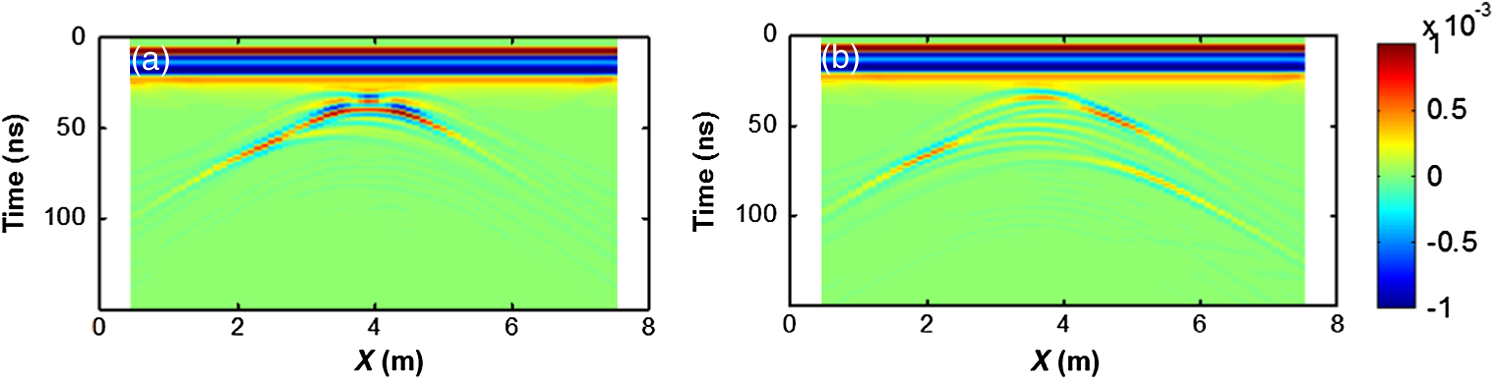
If the received GPR data have been amplified, the depth energy compensation algorithm will not be necessary. Otherwise, step 5 should be performed.

The aforementioned steps will be repeated until all the points in the imaging scene are considered.

3. Experimental Results and Analysis

To verify the performance of the proposed SBP algorithm, we design a synthetic and a practical field experiments for the objects imaging of complex shape. In addition, a serial contrast experiments are performed with the classic BP, the fast back projection (FBP)⁸, the SBP, and the 2-D depth migration algorithm with straight ray assumption.¹² To solve Eq. (2), the binary search algorithm is used by both the classic BP and SBP algorithms; the approximate algorithm proposed in Ref. 8 is used by the FBP algorithm. We evaluate the imaging error by the absolute cumulative error (ACE), which is defined as

Eq. (7)

δ_{ACE} = \sum_{}^{} | B - B^{*} | = \sum_{i} \sum_{j} | b_{i, j} - b_{i, j}^{*} |,

where

B

and

B^{*}

are the normalized matrices of the objects position matrix and imaging results matrix, and

b_{i, j}

and

b_{i, j}^{*}

are the elements in the matrices

B

and

B^{*}

, respectively. In this paper, all the programs are run by MATLAB 7.1 on the same hardware.

3.1.

Tests with Synthetic Data

According to Fig. 1, the geoelectric model of synthetic GPR data is formulated. The antennas are located 1 m above the surface of the surveyed structure. The scene is divided into two regions by $z = 0$ . The upper region is air with relative permittivity 1 and conductivity $0 S / m$ . The lower region is homogeneous medium with relative permittivity 16 and conductivity $0.001 S / m$ . The buried objects are shown in Fig. 2 by the blue curve with relative permittivity 9. The GPR wave fields of the geoelectric model are simulated by using a finite-difference time-domain¹³ solution of the Maxwell’s equations. In the synthetic experiment, a Ricker wavelet is taken as a pulse source with a center frequency of 100 MHz. The B-scans of the synthetic GPR data are shown in Fig. 3. By using the mean removal algorithm, we can preprocess the synthetic GPR data to suppress the interference partially from the terrain echo and the coupled wave between receiving and transmitting antennas. The normalized imaging results of the classic BP, the FBP, and the SBP are shown in Figs. 4, 5, and 6, respectively. The aforementioned imaging results are shown in Table 1. The velocity model of the 2-D depth migration algorithm is shown in Fig. 7, where the electromagnetic wave travels at $3 \times 10^{8} m / s$ in air and $7.5 \times 10^{7} m / s$ in earth, respectively. The normalized imaging results of the 2-D depth migration algorithm are shown in Fig. 8. The theoretical distributions of buried objects are labeled with the white circle curve, which is convenient to analyze the imaging results.

Table 1

Performance comparisons table about different imaging methods.

Imaging methods	y-shape object		z-shape object
Imaging methods	Absolute cumulative errors (ACEs)	Running times (s)	ACEs	Running times (s)
Classic back-projection	616.4	52.92	1017.4	52.95
FBP	250.3	3.71	471.1	3.72
SBP	28.9	2.53	51.6	2.54

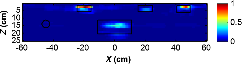
Fig. 2

Geoelectric models of the synthetic ground-penetrating radar (GPR) data: (a) $y$ -shape object and (b) $z$ -shape object.

Fig. 3

B-scans of the synthetic GPR data: (a) $y$ -shape object and (b) $z$ -shape object.

Fig. 4

Imaging result of the classic back-projection algorithm: (a) $y$ -shape object and (b) $z$ -shape object.

Fig. 5

Imaging result of the FBP algorithm: (a) $y$ -shape object and (b) $z$ -shape object.

Fig. 6

Imaging result of the self-correlation back-projection (SBP) algorithm: (a) $y$ -shape object and (b) $z$ -shape object.

Fig. 7

Velocity model of the two-dimensional (2-D) depth migration algorithm.

Fig. 8

Imaging result of the 2-D depth migration algorithm: (a) $y$ -shape object and (b) $z$ -shape object.

The experimental results show that the objects shape cannot be distinguished from Fig. 3. It may be recovered by the GPR signal-processing techniques. Due to the fact that buried objects have complex shapes in this experiment, each A-scan signal is the stack of multiple reflection echo signals. For a given imaging point, the echo information extracted by the BP algorithm from each A-scan signal may be the stack of the echo information of many imaging points. It reduces the imaging accuracy of the classic BP and FBP algorithms. For the same B-scan in GPR imaging, at the same condition of imaging resolution, the larger the number of the sensing locations, the longer the running time of both the BP and FBP algorithms. The SBP algorithm can adaptively choose the valid echo information sequence, with its running time related to the specific B-scan. The larger the number of the valid echo information sequence, the longer the running time of the SBP algorithm. However, the SBP algorithm usually has faster calculation speed because the valid echo information sequence is generally located in the multiple nearest neighbors of the imaging point. The 2-D depth migration algorithm can distinguish the objects shape effectively. However, the locations of the objects are moved upwards compared with their theoretical distribution. The GPR antennas and objects are distributed in different media. The precision of velocity model is reduced by the air between the GPR antennas and the earth. It is the main reason for the aforementioned imaging error. The experimental results illustrate that the proposed SBP algorithm is superior to the existing BP algorithms in terms of computing speed and imaging accuracy. Compared with the 2-D depth migration algorithm, the proposed SBP algorithm has a significant advantage in providing a rough outline of buried objects without prior knowledge of the velocity distribution.

3.2.

Field Test Case

The experimental data are collected at the Georgia Institute of Technology¹⁴ and is publicly available in Ref. 15 in MATLAB format files, and the field map in the detecting location is shown in Fig. 9. The data consist of different burial and no-object scenarios, and are taken with a multistatic stepped-frequency continuous-wave GPR. The GPR is scanned over a $1.8 m \times 1.8 m$ region at a constant height above the surface of the ground. The scan region is discretized into a grid of 91 points. At each scan position, GPR takes 401 equally spaced frequency measurements from 60 MHz to 8.06 GHz with 20-MHz increments. The pulse source is a differentiated Gaussian pulse with a center frequency of 2.5 GHz. The GPR B-scan is shown in Fig. 10, which is selected from the aforementioned experimental data. There are five buried objects at $- 45$ , $- 20$ , 0, 20, and 45 in cross-range ( $x$ ) dimension and $y = - 40$ . The distance between the transmitting and receiving antennas is 12 cm. The height of antennas is 27.8 cm above the surface of the surveyed structure. Each A-scan is acquired every 2 cm. The electromagnetic wave travels at $2.998 \times 10^{8} m / s$ in air and $1.5 \times 10^{8} m / s$ in sand.¹⁶ The field GPR data are preprocessed by the removing mean value method to suppress the interference partially from the terrain echo and the coupled wave between receiving and transmitting antennas. The normalized imaging result of the SBP algorithm is shown in Fig. 11. The theoretical distributions of buried objects are labeled with the black curve, which is convenient to analyze the imaging results.

Fig. 9

Field maps in the detecting location.¹⁶

Fig. 10

B-scan of the field GPR data.

Fig. 11

Imaging result of the SBP algorithm.

The experimental result shows that the proposed SBP algorithm can effectively recover the multiple objects’ position information. The calculated ACE for Fig. 11 is 426.5, and the running time of the SBP algorithm is 3.5 s. It further validates the effectiveness of the proposed SBP algorithm.

4. Conclusion

Based on the existing BP algorithms, the SBP algorithm is proposed in this paper, which can reconstruct the shape of buried objects in GPR imaging. By setting up the correlation threshold, the SBP algorithm can adaptively choose the valid echo information sequence of the imaging points, which improves the image resolution. Because the valid echo information sequence is generally located in the multiple nearest neighbors of the imaging point, the SBP algorithm usually has a faster calculation speed. In addition, the imaging result is postprocessed by the depth energy compensation algorithm to improve the imaging resolution. The experimental results show that the SBP algorithm is superior to the classic BP and FBP algorithms in terms of computing speed and imaging accuracy. It has a significant advantage in providing a rough outline of buried objects without prior knowledge of the velocity distribution. The application of the proposed SBP algorithm is valuable in the imaging of underground objects with fast speed and high quality.

Acknowledgments

This work was funded by the National Natural Science Foundation of China (Nos. 61102115, 61362020, and 61371186), the Natural Science Foundation of Guangxi Province (Nos. 2012GXNSFBA053177, 2013GXNSFAA019327, and 2013GXNSFFA019004), and the Guangxi Experiment Center of Information Science, Guilin University of Electronic Technology (No. 20130112).

References

1.

A. Tzanis, “Detection and extraction of orientation-and-scale-dependent information from two-dimensional GPR data with tuneable directional wavelet filters,” J. Appl. Geophys., 89 48 –67 (2013). http://dx.doi.org/10.1016/j.jappgeo.2012.11.007 JAGPEA 0926-9851 Google Scholar

2.

H. Zhang et al., “Matched filtering algorithm based on phase-shifting pursuit for ground-penetrating radar signal enhancement,” J. Appl. Remote Sens., 8 (1), 083593 (2014). http://dx.doi.org/10.1117/1.JRS.8.083593 Google Scholar

3.

J. Yang et al., “Sparse MIMO array forward-looking GPR imaging based on compressed sensing in clutter environment,” IEEE Trans. Geosci. Remote Sens., 52 (7), 4480 –4494 (2014). http://dx.doi.org/10.1109/TGRS.2013.2282308 IGRSD2 0196-2892 Google Scholar

4.

S. H. H. Lum, T. Tang and J. Lyall, “Improved GPR image quality by truncating the bandwidth of the Fourier transform in 2D diffraction tomographic inversion,” in IEEE Int. RF and Microwave Conf., 391 –394 (2008). Google Scholar

5.

M. Razavian, M. H. Hosseini and R. Safian, “Time-reversal imaging using one transmitting antenna based on independent component analysis,” IEEE Geosci. Remote Sens. Lett., 11 (9), 1574 –1578 (2014). http://dx.doi.org/10.1109/LGRS.2014.2301724 Google Scholar

6.

L. Zhou and Y. Su, “GPR imaging with RM algorithm in layered mediums,” IEEE Geosci. Remote Sens. Lett., 8 (5), 934 –938 (2011). http://dx.doi.org/10.1109/LGRS.2011.2138116 Google Scholar

7.

B. Hua and G. A. McMechan, “Parsimonious 2D prestack Kirchhoff depth migration,” Geophysics, 68 (3), 1043 –1051 (2003). http://dx.doi.org/10.1190/1.1581075 GPYSA7 0016-8033 Google Scholar

8.

L. Zhou, C. Huang and Y. Su, “A fast back-projection algorithm based on cross correlation for GPR imaging,” IEEE Geosci. Remote Sens. Lett., 9 (2), 228 –232 (2012). http://dx.doi.org/10.1109/LGRS.2011.2165523 Google Scholar

9.

A. Tzanis, “The curvelet transform in the analysis of 2-D GPR data: signal enhancement and extraction of orientation-and-scale-dependent information,” J. Appl. Geophys., 115 145 –170 (2015). http://dx.doi.org/10.1016/j.jappgeo.2015.02.015 JAGPEA 0926-9851 Google Scholar

10.

Y. Zhang and T. Xia, “OFDM and compressive sensing based GPR imaging using SAR focusing algorithm,” Proc. SPIE, 9437 943725 (2015). http://dx.doi.org/10.1117/12.2083857 PSISDG 0277-786X Google Scholar

11.

Y. Zhang et al., “Data analysis technique to leverage ground penetrating radar ballast inspection performance,” in 2014 IEEE Radar Conf., 463 –468 (2014). Google Scholar

12.

B. Biondi and T. Tisserant, “3D angle-domain common-image gathers for migration velocity analysis,” Geophys. Prospect., 52 (6), 575 –591 (2004). http://dx.doi.org/10.1111/j.1365-2478.2004.00444.x GPPRAR 0016-8025 Google Scholar

13.

G. R. Werner, C. A. Bauer and J. R. Cary, “A more accurate, stable, FDTD algorithm for electromagnetics in anisotropic dielectrics,” J. Comput. Phys., 255 (12), 436 –455 (2013). http://dx.doi.org/10.1016/j.jcp.2013.08.009 JCTPAH 0021-9991 Google Scholar

14.

A. C. Gurbuz, “Determination of background distribution for ground-penetrating radar data,” IEEE Geosci. Remote Sens. Lett., 9 (4), 544 –548 (2012). http://dx.doi.org/10.1109/LGRS.2011.2174137 Google Scholar

15.

W. R. Scott, “Multistatic ground-penetrating radar experiments,” (2007) http://users.ece.gatech.edu/~wrscott/ Google Scholar

16.

T. Counts et al., “Multistatic ground-penetrating radar experiments,” IEEE Trans. Geosci. Remote Sens., 45 (8), 2544 –2553 (2007). http://dx.doi.org/10.1109/TGRS.2007.900677 IGRSD2 0196-2892 Google Scholar

Biography

Hairu Zhang received his BEng degree from Wuhan University of Science and Technology, Wuhan, China, in 2009 and obtained his MEng degree from Guilin University of Electronic Technology, Guilin, China, in 2012. Currently, he is a PhD student at Xidian University, Xi’an, China. His fields of interest include signal processing for ground-penetrating radar, computational intelligence, and adaptive signal processing.

Shan Ouyang received his BEng degree from Guilin University of Electronic Technology, Guilin, China, in 1986 and obtained his MEng and PhD degrees in electronic engineering from Xidian University, Xi’an, China, in 1992 and 2000, respectively. He received the National Excellent Doctoral Dissertation of China in 2002. Currently, he is a professor and PhD supervisor at Guilin University of Electronic Technology. His fields of interest include signal processing for communications and radar.

Guofu Wang received his BEng degree from Wuhan University of Technology, Wuhan, China, in 2002 and obtained his MEng and PhD degrees from Xi’an Institute Optics and Precision Mechanics of CAS, Xi’an, China, in 2005 and 2007, respectively. Currently, he is a professor at Guilin University of Electronic Technology. His fields of interest include signal processing for ground-penetrating radar and adaptive signal processing.

Jingjing Li received his BEng degree from Henan Polytechnic University, Jiaozuo, China, in 2010 and obtained his MEng degree from Guilin University of Electronic Technology, Guilin, China, in 2014. Currently, she is a PhD student at Guilin University of Electronic Technology, Guilin, China. Her fields of interest include signal processing for radar.

Biographies for the other authors are not available.

CC BY: © The Authors. Published by SPIE under a Creative Commons Attribution 4.0 Unported License. Distribution or reproduction of this work in whole or in part requires full attribution of the original publication, including its DOI.

Citation Download Citation

Hairu Zhang, Ouyang Shan, Guofu Wang, Jingjing Li, Suolu Wu, and Faquan Zhang "Back-projection algorithm based on self-correlation for ground-penetrating radar imaging," Journal of Applied Remote Sensing 9(1), 095059 (24 July 2015). https://doi.org/10.1117/1.JRS.9.095059

Published: 24 July 2015

Access the abstract

JOURNAL ARTICLE
10 PAGES

DOWNLOAD PAPER SAVE TO MY LIBRARY

GET CITATION

CITATIONS

Cited by 13 scholarly publications.

Explore citations on Lens.org

KEYWORDS

General packet radio service

Radar imaging

Antennas

Ground penetrating radar

Image resolution

Detection and tracking algorithms

Data modeling

1.

Introduction

2.

Self-Correlation Back-Projection Algorithm

Fig. 1

2.1.

Two-Way Traveltime

Eq. (1)

Eq. (2)

Eq. (3)

2.2.

Self-Correlation Back-Projection Algorithm Developing Steps

Eq. (4)

Eq. (5)

Eq. (6)

3.

Experimental Results and Analysis

Eq. (7)

3.1.

Tests with Synthetic Data

Table 1

Fig. 2

Fig. 3

Fig. 4

Fig. 5

Fig. 6

Fig. 7

Fig. 8

3.2.

Field Test Case

Fig. 9

Fig. 10

Fig. 11

4.

Conclusion

Acknowledgments

References

Biography

Show All Keywords

Keywords/Phrases

Search In:

Publication Years