1.

Introduction

Concentrated solar power (CSP) is expected to grow as a clean and affordable source of energy in the next few decades. Studies¹ have shown that solar energy can be used to supply up to 35% of the total energy requirements by 2050 with huge reductions in greenhouse gas emissions. Nine CSP plants² were built in the time period from 1980 to 1990 with a total capacity of 354 MW. This was followed by a period of skepticism about the viability of solar power generation. In 2000, the National Academies’ National Research Council³ recommended that the Solar Energy Technologies Program should abandon further research and development of solar technologies as it would not lead to deployment and there was not enough economic scope in such a deployment. This was followed by a U.S. Department of Energy report² in 2002, which concluded that with proper government incentives, over 1000 MW of solar power could be generated within a 10- to 20-year time frame. Due to the conflicting conclusions of the reports, DOE hired an independent firm to assess the feasibility of solar power plants in the US. The firm again concluded that CSP is economically feasible and viable if taken up on a large scale.⁴

The interest in CSP has been revived again and the US Department of Interior approved the largest solar energy project to be built on public lands in Riverside, California, in October 2010. With its vast expanse of lands, especially in the western half of the country, the US has a huge potential for CSP. The first task in building CSP is to identify potential sites where these plants can be built, and it is no surprise that GIS has been used in some of the national evaluations for CSP locations.⁵ Available tools include a GIS map,⁶ which allows a static view of a few map layers overlaid on top of each other. GIS modeling and analysis would be the best tool to delineate sites for CSP locations, since these plants are expected to be built on unused, degraded, or marginal lands where GIS modeling can be very useful for locating the sites. GIS modeling enables the combination of environmental parameters (e.g., solar radiation, water availability) with physical parameters (e.g., land use, land cover, etc.) and the infrastructure facilities (e.g., roads, grid lines, etc.) to identify suitable lands for siting CSP plants.

GIS modeling has traditionally been used for site selection but not much work has been done in locating sites for large-scale solar plants. A survey of literature indicates the modeling of solar radiation advanced very rapidly starting from 1980 and by the late 1990s models, such as SolarFlux, Genasys Solar Analyst, and r.sun, were available in open and commercial GIS packages which could very accurately estimate solar radiation at various spatial and temporal resolutions. However, there is a lack of good modeling tools to site CSP plants even though the concept has gained importance recently due to concerns of depleting fossil fuels, greenhouse gas emissions, and the political instability in some of the regions which are the highest producers of oil and gas. In the following section, an exhaustive literature review has been provided which traces the development of solar radiation models followed by some very recent work on locating CSP locations.

2.

Literature Review

Gautier et al.⁷ were one of the first to develop a simple physical model to estimate surface solar radiation from geostationary operational environmental satellite satellite data. This physical model used satellite data to calculate incident solar radiation for an area of interest and it provided a quick and fast estimation of solar radiation over large areas. This had a distinct advantage over using conventional pyrometer networks in that it provided better temporal and spatial resolution, while the advantage of using a physical model over a statistical one was that it allowed continuous modeling of the surface rather than doing it on smaller discreet regions. These models were refined over time by Cano et al.,⁸ Beyer et al.,^9,10 and Becker.¹¹ These led to more accurate estimation of solar radiation as the refined models had better algorithms and used more variables to calculate solar radiation.

SolarFlux¹² was one of the first solar radiation models that were developed and it was developed on the ARCINFO platform. Compared to the previous solar radiation models which allowed the users to estimate solar radiation values based primarily on satellite data, SolarFlux provided users with the flexibility to model solar radiation based on various parameters like surface orientation, time interval and spatial coordinates. Arc Marco Language was used to develop the programming environment and consisted of four modules to perform four tasks, which were later integrated into a single model. These were followed by development of Genasys¹³ and Solei,¹⁴ which was linked to the GIS software IDRISI. These models used digital elevation models (DEMs) to calculate solar radiation and enabled the users to perform statistical calculations.

The first independent modeling tool was developed as an ArcView GIS extension module.¹⁵ Instead of using the simple interpolation techniques used in the previous models, they used optimized algorithms to account for influences of viewshed, surface orientation, elevation, and atmospheric corrections. The Solar Analyst combined the strengths of both point and area-based models and enabled the user to create maps of direct, diffuse and global radiation for various time resolutions. It also allowed viewers to calculate viewsheds and horizon angles. The interface with ArcView software enabled querying, graphing and statistical analysis. The model generated an upward looking hemispherical viewshed based on a digital terrain model. Some of the inputs required for the model included a DEM, spatial coordinates of the study area, sky size, transmittivity, and time configuration.

In 2004, Suri and Hofierka¹⁶ developed a GIS model known as r.sun which runs on the open source GRASS GIS software; this was an extension of the earlier work of Hofierka.¹⁷ The model enabled users to calculate all three components of the solar irradiance for clear as well as cloudy skies, whereas previous Hofierka’s earlier model did not allow for calculations of atmospheric transmissivity and the diffuse proportions. The r.sun model worked in a two-mode system: in mode 1, it created rasters of selected components of solar irradiance for a particular time; whereas in mode 2, it created daily raster maps which are based on the integration of irradiance values. The model required fewer input parameters and derived the remaining parameters from the given inputs, thus allowing users to model at different scales ranging from local to global. The model was found to be very sensitive to elevation effects and viewshed directions. The r.sun model has been expanded¹⁸ to take into consideration 3-D surfaces like facades and shadows which capture the temporal and spatial variation of solar radiation in urban environments with tall buildings. More recently, r.sun has been coupled with a canopy openness index derived from light detection and ranging (LiDAR) data to produce a subcanopy solar radiation model.¹⁹

Recently, Kodysh et al.²⁰ presented a methodology that advances previous efforts by estimating solar radiation potentials on multiple rooftops in an urban area for photovoltaic (PV) applications using DEM from LiDAR data and an upward looking hemispherical algorithm. Their methodology considers input parameters such as surface orientation, shadowing effect, elevation, and atmospheric conditions that influence solar intensity on the Earth’s surface; it was implemented for some 212,000 buildings in Knox County, Tennessee, United States.

Once solar GIS models were developed, solar radiation maps for a particular region could be easily and accurately calculated. As technology moved forward, the focus shifted from single PV installations which could power individual houses or street lights, to larger CSP plants which could: (a) produce larger amounts of power; (b) be operational after sunset; and (c) could be connected to the national grid. This called for the development of siting models, which could take in various parameters and produce optimal sites for construction of CSP plants.

The work of Broesamle²¹ was one of the first which used GIS modeling to assess the solar electricity potential in North Africa. Unlike earlier studies which focused more on estimating solar radiation, this work was focused on selecting sites in North Africa where solar thermal power plants could be located. The system that developed was known as STEPS, which consisted of a main module and five-linked submodules. The main module allowed users to control spatial and temporal resolutions along with some environmental analysis. The submodules were used to: (1) assess geographical conditions, (2) assess meteorological conditions, (3) load country infrastructure database, (4) perform economic analysis, and (5) perform power block simulation. This model was the first to use a variety of input data and integrate them to produce siting results. Geographic data used in this model included land use/land cover data, DEM and slope. The model enabled users to perform solar radiation resource assessment using meteorological data, simulate power plant performance and provide a cost estimate of a solar thermal power plant. It also allowed users to calculate infrastructure costs based on distances from roads, power lines, and the availability of water for cooling. Broesamle et al.²² extended this framework to include desalination plants along with solar plants for the Mediterranean region. Additional variables were included in the siting study, including risk factors and performance parameters for CSP plants.

Carrion et al.²³ developed a decision support system for optimal site selection for grid-connected PV power plants. They used environmental, orography, location, and climate criteria to build the decision support system. Their model used a system which was based on multicriteria analysis (MCE) with a single objective and several criteria. They used an analytic hierarchy process developed by Saaty²⁴ to assign weights to each criteria, factor and indicator. This enabled them to determine the relative importance of each factor and criteria for selection of solar sites, thus weights could be assigned based on their relative importance. They also used the consistency ratio to determine if the values were sufficiently consistent to establish the weights. Once weights were determined, the criteria and factors were ordered according to their degree of importance and then normalized on a scale of 1 to 10. These normalized values were then used to make a model using Model Builder in ArcView.

With reference to the studies of identifying suitability sites for CSP plants in the US, Fthenakis et al.¹ did a technical, geographical and economical feasibility study which was more statistical in nature. Using past statistical solar radiation data and worst case climate scenarios, they showed that CSP would be economically viable in the US by 2020. They also performed an economic analysis to predict future costs of solar power generation for the next 50 years and showed that it had the potential to meet most of the energy demands of the US based on land and solar radiation supplies in the southwest. Fadare et al.²⁵ used artificial neural networks to model solar potential studies in Africa. Using satellite data for 172 locations for a period of 22 years and geographical and meteorological data, they produced monthly solar radiation intensity maps. They used a multilayer, feed-forward and back-propagation network consisting of three layers for their model.

As the CSP technology advances, there are not many models or tools which can be used to assess the availability of sites for CSP on a variety of scales starting from local to global. However, a few recent studies have attempted to do so in localized regions. Anders et al.²⁶ did a study for the San Diego region, whereas Bravo et al.²⁷ did studies in Spain; Fluri²⁸ did a study for South Africa; and Clifton and Boruff²⁹ have also used GIS tools to estimate areas of potential CSP development in rural regions of western Australia. Gastli et al.³⁰ did a GIS-based assessment of a CSP plant in Duqum, Oman. All these models used very simple overlay techniques to estimate areas for optimal location of power plants; the only difference in these studies are the number of layers used (minimum 5, maximum 10) for determining suitable sites.

A different approach was used by Badran et al.³¹ who used fuzzy logic to assess solar sites in Jordan. Using fuzzy logic, the authors could best estimate benefit and cost parameters for siting CSP plants. Janke,³² on the other hand, used multicriteria analysis to locate wind and solar farms in the state of Colorado. Datasets, including solar potential (obtained from the National Renewable Energy Laboratory, land cover, distance to roads, population density, and distance to transmission line) were scaled from 0 to 1 with a gradational rating of excellent to poor and overlaid to produce maps which showed the suitability of areas for wind and solar farms. Comparison of existing facilities showed that the wind farm locations matched the model while there was poor correlation between existing solar facilities and predicted areas. This could be due to the fact that solar facilities were not planned properly or the model needs to be reevaluated for its effectiveness.

3.

Methodology

The methodology presented here is a two-stage process. First, global solar radiation in $\mathrm{Wh}/{\mathrm{m}}^2/\mathrm{day}$ is calculated using the satellite data obtained from the National Aeronautical and Space Administration (NASA) Global Energy and Water Cycle (GEWEX) for the entire continental United States. Second, using eight metrics defined for some 30 GIS data sets and a grid divided into 100 m cells, the study area is classified with respect to its degree of site suitability. Based on these outputs, two applications of solar power plants are analyzed.

4.

Results

Figure 1 shows the average global solar radiation for the winter (a) and summer (b) months. According to the data, we can easily conclude that using the results for the summer months is a good representation of the average global solar radiation and that setting the minimum global solar radiation at $4.8\mathrm{kWh}/{\mathrm{m}}^2/\mathrm{day}$ for one case and $6.0\mathrm{kWh}/{\mathrm{m}}^2/\mathrm{day}$ for another case provides an opportunity to explore potential land areas all over the CONUS.

Fig. 1

Average global solar radiation for the (a) winter months (December, January, and February) and (b) summer months (June, July, and August), respectively.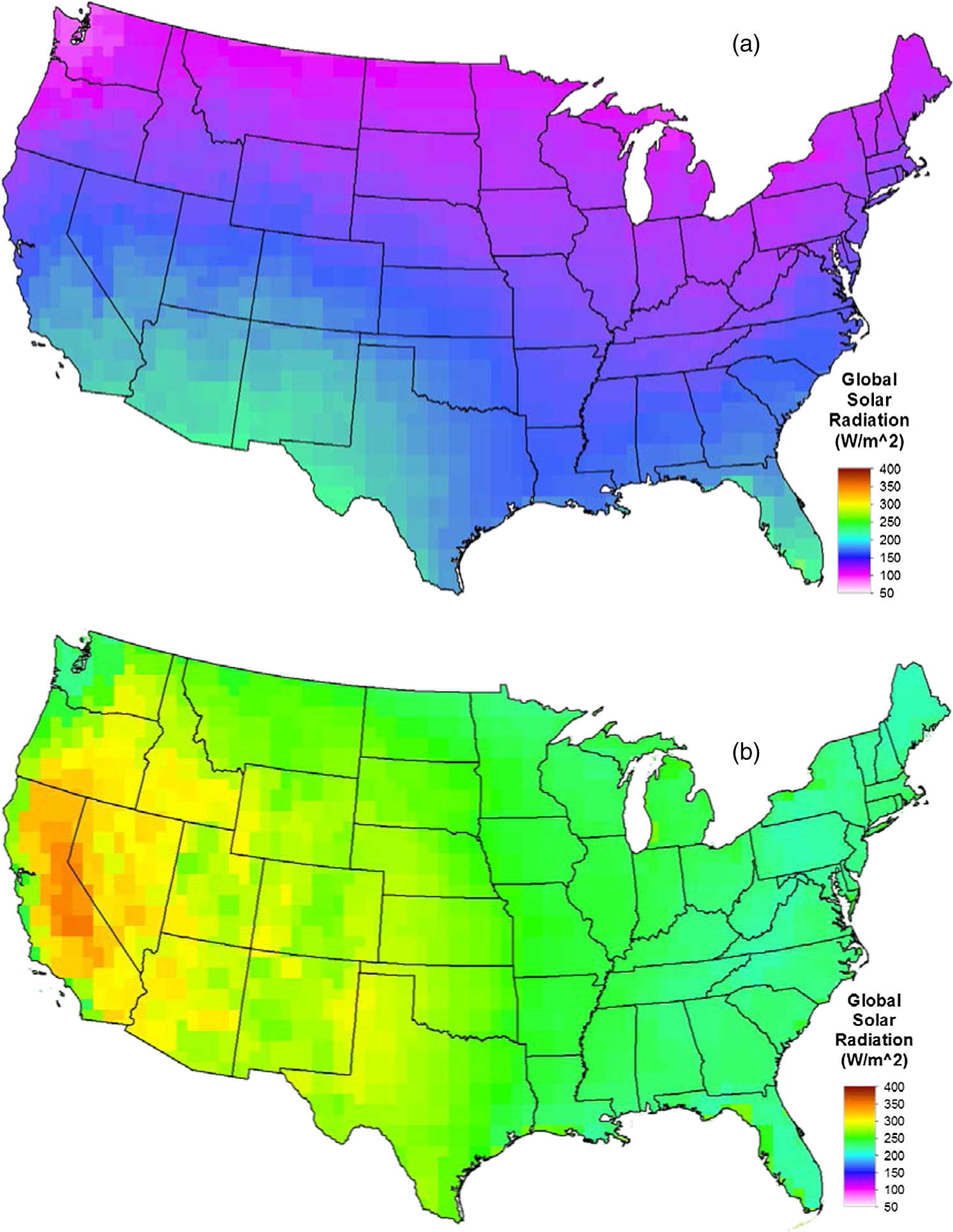

The excluded data layers for these two cases based on the solar radiation metric are shown in Fig. 2. Excluded areas are areas that are not suitable for siting CSP based on the criteria for the respective metric (fail) and nonexcluded areas are areas that are suitable for siting CSP based on the criteria for the respective metric (pass).

Fig. 2

Excluded solar radiation data layers. (a) Minimum global solar radiation set at $4.8\mathrm{kWh}/{\mathrm{m}}^2/\mathrm{day}$. (b) Minimum global solar radiation set at $6.0\mathrm{kWh}/{\mathrm{m}}^2/\mathrm{day}$.

The excluded areas and nonexcluded areas for each of the other metrics are shown in Fig. 3.

Fig. 3

Individual data layers representing the other seven metrics for CSP site suitability in the following order: (a) population, (b) protected lands, (c) wetlands and open water, (d) landslide hazards, (e) 100-year floodplain, (f) 5% slope, and (g) $\mathrm{15,000}\mathrm{gallons}/\min$ stream flow.

4.1.

Suitability Areas for CSP Plants that Drive Steam Turbine

An algebraic combination of the data layers representing all the metrics resulting in the outputs is shown in Fig. 4. The green areas are areas that meet all metrics threshold and are completely suitable. The other areas are partially suitable because they failed in at least one metric as follows: the yellow areas are areas that failed on one or two metrics; gold areas failed on three or four metrics; and purple areas failed on at least five metrics. Let us call the results obtained by setting the minimum global solar radiation at $4.8\mathrm{kWh}/{\mathrm{m}}^2/\mathrm{day}$ our case-1 and the results obtained by setting the minimum global solar radiation at $6.0\mathrm{kWh}/{\mathrm{m}}^2/\mathrm{day}$ are our case-2.

Fig. 4

Results of the map algebra of the eight metrics for CSP (wet options) with (a) global solar radiation set at $4.8\mathrm{kWh}/{\mathrm{m}}^2/\mathrm{day}$ and (b) global solar radiation set at $6.0\mathrm{kWh}/{\mathrm{m}}^2/\mathrm{day}$.

The green areas for case-1 represent 28.1% of the total land area in CONUS and 10.9% of the total land area for case-2. The difference in land area between the two cases is more than 17%, which is almost two times the size of the suitable land area for case-2. One implication of these results is that with improved technology that could make lower global solar radiation more economical for CSP applications, more land areas, especially in the eastern half of CONUS, could become more suitable. Looking at the results for case-2, most of the suitable land areas are in the midwestern states from Texas to North Dakota. Some of these areas may also be suitable for other renewable or no-carbon energy sources, such as wind and natural gas. Hence, different energy sources may be competing for land in these areas. On the other hand, the impact of climate change with regard to seasonal drought is another concern for these areas. Our future studies in this area will model the implications of these interdependencies.

4.2.

Suitability Areas for CSP Plants that Drive Sterling Engine

Looking at the results in Fig. 4, we can conclude that one of the two major limiting factors is cooling water. Therefore, if we perform a sensitivity analysis by not including the streamflow metric, that is considering CSP plants that drive a Sterling engine, the outputs of the algebraic combination of the data layers are shown in Fig. 5. The different colors have the same interpretation as the outputs in Fig. 4. The green areas for case-1 for the Sterling application represent about 43.5% of the total CONUS land area; for case-2, it is about 24.3%. The difference in suitable land area for this application is about 19%, almost the same as the land area for case-2.

Fig. 5

Results of the map algebra of the eight metrics for CSP (dry options) with (a) global solar radiation set at $4.8\mathrm{kWh}/{\mathrm{m}}^2/\mathrm{day}$ and (b) global solar radiation set at $6.0\mathrm{kWh}/{\mathrm{m}}^2/\mathrm{day}$.

5.

Conclusions

The increasing environmental cost of fossil fuels is driving policy makers in the United States to promote electricity generation from renewable energy sources, such as solar. We have presented a methodology for identifying a CSP siting suitability index for the contiguous United States. This is achieved by dividing the entire country into a grid of 100-m cells. We proposed eight metrics that use about 30 GIS data layers to characterize each cell and identify areas with the highest suitability index. The solar radiation potential data uses a remote sensing data derived from the NASA/GEWEX (Global Energy and Water Cycle) Surface Radiation Budget project. The methodology was implemented for two applications of CSPs—CSPs that drive steam turbines and CSPs that drive a Sterling engine. The results show that about 11% and 24%, respectively, of the CONUS area have the highest suitability index for CSP (steam turbine and Sterling engine) applications if the minimum global solar radiation is set at $6.0\mathrm{kWh}/{\mathrm{m}}^2/\mathrm{day}$, whereas, about 28% and 44%, respectively, of the CONUS area have the highest suitability index for the two CSP applications if the minimum global solar radiation is set at $4.8\mathrm{kWh}/{\mathrm{m}}^2/\mathrm{day}$.