1.

Introduction

There has been a significant effort to describe passive remote sensor signals for case 1 waters with a semianalytic approach.^1–8 For case 1 waters, the optical properties are assumed to be dominated by pure water contributions and the effects of chlorophyll-containing phytoplankton. In the semianalytic approach, analytic relationships between optical properties of the water are combined with empirical dependencies on chlorophyll concentration. In these studies, the optical properties are assumed to be homogeneous, determined by the value of chlorophyll concentration at the surface.

More recently, the approach has been extended to include case 2 waters,^9–13 generally coastal waters, where the effects of suspended and dissolved materials that are not related to chlorophyll on the optical properties are important. In these investigations, the main motivation was the estimation of chlorophyll concentration from passive remote sensing signals in coastal and estuarine waters.

Other work has focused on deriving additional information from passive remote sensors. One area of investigation has been to obtain information about phytoplankton cell size.^14–17 Another is to identify phytoplankton functional groups.^18–21 A third area is to detect harmful algal blooms.^22–25

There have been several investigations into the effects of nonuniform vertical distribution of chlorophyll on passive remote sensing signals. Sathyendranath and Platt²⁶ investigated the effects on the blue-green ratio and found relative errors in excess of 100% in estimates of photic depth and total chlorophyll concentration in the photic zone. Gordon²⁷ used a Monte-Carlo simulation to test the hypothesis that the reflectance of a stratified ocean is the same as that of a homogeneous ocean with a constant chlorophyll concentration equal to the depth-weighted average of the actual profile, and found that the hypothesis was accurate to within 25% for the cases tested. Stramska and Stramski²⁸ used a sophisticated radiative transfer model to investigate the effects of a nonuniform depth profile, reporting differences from the uniform profile greater than 70%, with the larger differences produced by lower surface chlorophyll concentrations. Pitarch et al.²⁹ considered retrieval of the chlorophyll profile using passive remote sensing with some success.

Approximate models of active remote sensor signals have also been developed.³⁰ The most successful is probably the quasisingle-scattering approximation,^2,31–33 which has been shown to provide good agreement with measured values.³⁴ This model has recently been used to obtain an expression for the lidar extinction-to-backscatter ratio for lidar inversions³⁵ that can provide the depth profile of phytoplankton directly.

Roughly, half of the global photosynthesis takes place in the upper ocean, and inversion models have been developed to quantify this production using satellite data.^36–38 These models are generally based on surface chlorophyll concentration from ocean color and sea-surface temperature from thermal radiometers. These estimates do not always agree with in situ estimates of productivity, and stratification has been suggested as one possible reason for the discrepancy.³⁸

Stratification is important, because phytoplankton are often seen to occur in thin (3 to 5 m or less) layers associated at the pycnocline at the base of the surface mixed layer.^39–41 Most of the observations have been in coastal regions, but thin layers have also been observed in the open ocean.³⁹ These layers can contain a significant fraction of the total chlorophyll in the water column,^42,43 affecting not only primary production, but also the grazing success of zooplankton and higher-trophic levels.

In this work, we consider a semianalytic bio-optical model to describe passive and active remote sensor signals. To illustrate the effects of stratification, a layer of relatively high-chlorophyll concentration is embedded within a lower-background concentration. The effects of such a layer on primary productivity and on satellite estimates of primary productivity are estimated.

2.

Semianalytic Bio-Optical Model

In the semianalytic ocean color model of Gordon et al.,¹

For passive remote sensing, we are interested in the remote sensing reflectance, $R_{\mathrm{rs}}$, defined as the ratio of the upwelling radiance to the downwelling irradiance just above the surface. Mobley⁴⁴ has shown that $R_{\mathrm{rs}}$ can be approximated by $0.54R/Q$, so we have

We can relate the remote sensing reflectance to chlorophyll concentration, $C$, using the model described by Morel and Maritorena.³ In this model, we have

Morel and Maritorena³ also present a model for diffuse attenuation given by

The number of segments, the degree of the polynomials, and the number of significant digits for the coefficients have been selected so that the errors in chlorophyll concentration produced by this approximation are 10% or less. The resulting error in the estimate of $K_d$ is plotted in Fig. 1. The errors are all less than 5%, except for very low-chlorophyll concentration near the minimum absorption. Here, $K_d$ is very small and the errors are dominated by those in our estimate of $K_w$. The root-mean-square error for all values is 2.2%.

Fig. 1

Relative error in $K_d$ estimated from Eqs. (10)–(12), relative to that using the tabulated values for chlorophyll concentrations of $C=0.01(+)$, 0.1 (×), 1 (○), a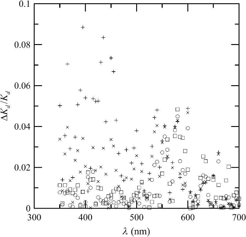nd 10 (□) $\mathrm{mg}{\mathrm{m}}^{-3}$.

Several examples of remote sensing spectra (Fig. 2) confirm that the values are generally below $0.01{\mathrm{sr}}^{-1}$, and the second term in Eq. (1) can be neglected. These examples also show that the piecewise polynomial fit reproduces the remote sensing reflectance spectra obtained from the tabulated parameters.

Fig. 2

Remote sensing reflectance, $R_{\mathrm{rs}}$, versus wavelength, $\lambda$, for the tabulated parameters (solid lines) and the piecewise polynomial fit (dashed lines) for several values of chlorophyll concentration $C$.

For active remote sensing, similar expressions can be used. We will restrict ourselves to a broad-beam, unpolarized lidar for which the received signal can be written as^30,33

There are two reasons for preferring a broad beam. The primary one is that it provides the minimum attenuation possible at a given wavelength,^30,32 which results in the maximum penetration depth. This is a consequence of the distribution of particulate scattering in the ocean, which is dominated by scattering at small angles. Most scattered light will remain within a broad beam, and not contribute to attenuation. For a narrow beam, this light will be scattered outside of the beam, and does contribute to overall attenuation. A secondary advantage is that a broader beam is less likely to pose a laser-exposure risk.⁴⁸

The only reason to consider unpolarized lidar is that we do not currently have a good model for polarization characteristics. This is an area that deserves more attention, since layers are much more detectable by polarization lidar.^34,39,49,50

3.

Estimating Chlorophyll

The operational chlorophyll algorithms have the form

Fig. 3

Estimated chlorophyll concentration, $C_{\mathrm{est}}$, as a function of the concentration used in the bio-optical model, $C$, for the OC3M algorithm (long dashes) and the modified algorithm of Eq. (17) (solid line). Short dashes provide the desired one-to-one relationship.

The OC3M algorithm can be modified to fit our bio-optical model, with the result

To estimate $C$ from 532 nm lidar data, we will use the modified lidar extinction-to-backscatter ratio³⁵

The actual estimate of $C$ can be found iteratively. We begin with a value of $S=100$ and calculate $C_{\mathrm{est}}$. That value is used to calculate a new estimate for $S$ from Eq. (19), which is used to calculate a new $C_{\mathrm{est}}$. The first estimate is close to the actual value for small concentrations (Fig. 4). By the 10th iteration, the estimate is within 2.5% of the actual value, even for very high values of $C$. To obtain depth profiles, one starts at the surface sample and works progressively deeper, using the estimated attenuation profile to obtain the actual value of $\beta$ from the measured signal at each depth.

Fig. 4

Estimated chlorophyll concentration, $C_{\mathrm{est}}$, as a function of the concentration used in the bio-optical model, $C$, for the iterative lidar inversion. The short dashed line is the first estimate, the long dashed line is the second estimate, and the solid line is the 10th estimate, which is indistinguishable from the actual value.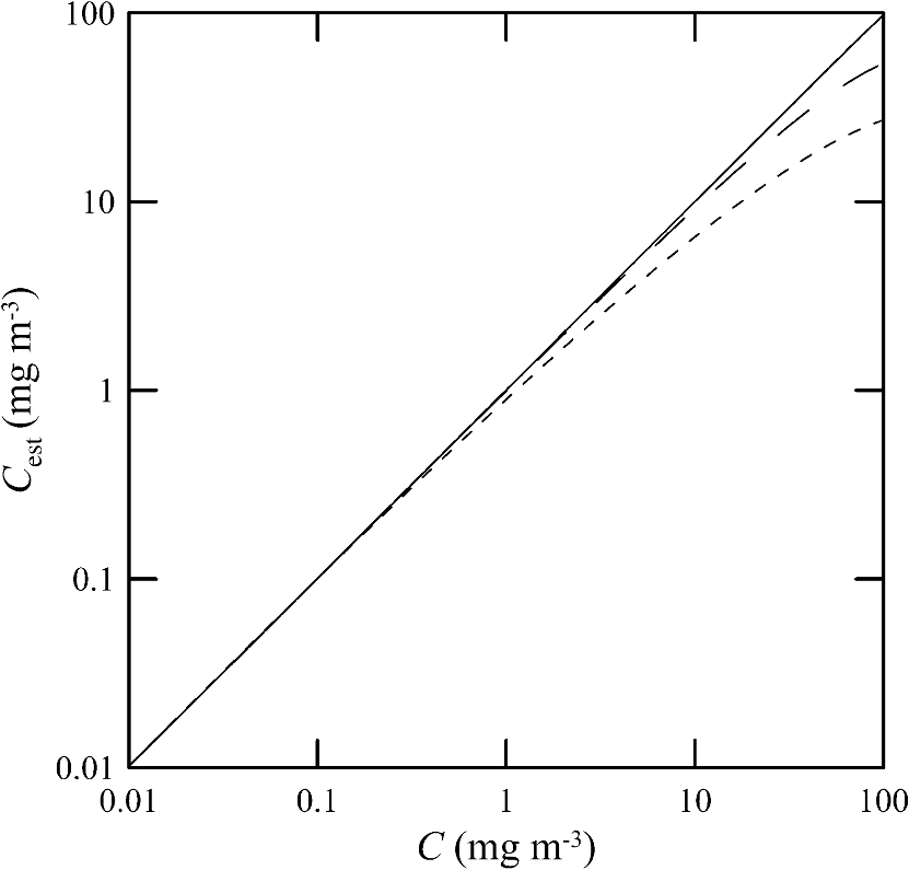

4.

Primary Productivity

We can investigate the effects of thin layers on primary productivity using a model based on chlorophyll concentration.^36,37 We will use the vertically generalized production model, which takes the form

Surface PAR was estimated using MODTRAN4⁵³ with no clouds and the appropriate standard aerosol model. For the example of year day 180 and latitude of 45°N, this would be the midlatitude summer model. Values were integrated over the 400 to 700 nm PAR band and over daylight hours. Subsurface values were estimated using an assumed attenuation coefficient of⁶

Behrenfeld and Falkowski³⁷ concluded that replacing the chlorophyll profile by the surface concentration produces acceptable results. In this case, satellite estimates of surface chlorophyll concentration, aerosol optical depth, and sea-surface temperature can provide global estimates of oceanic primary productivity using the approximate equation

5.

Stratified Water Example

To illustrate the effects of stratification, we will consider the case of a layer of water with $C=C_l$ within region with a background level, $C=C_b$. The top of the layer is at depth $z_0$ and the bottom at $z_1$ (Fig. 5). For this geometry, it is straightforward to perform the integrations in Eq. (5), with the result

Fig. 5

Schematic of layer used for calculations. A layer with chlorophyll concentration $C_l$ and thickness $L$ is located with its top at a depth $z_0$. Background chlorophyll concentration above and below the layer is 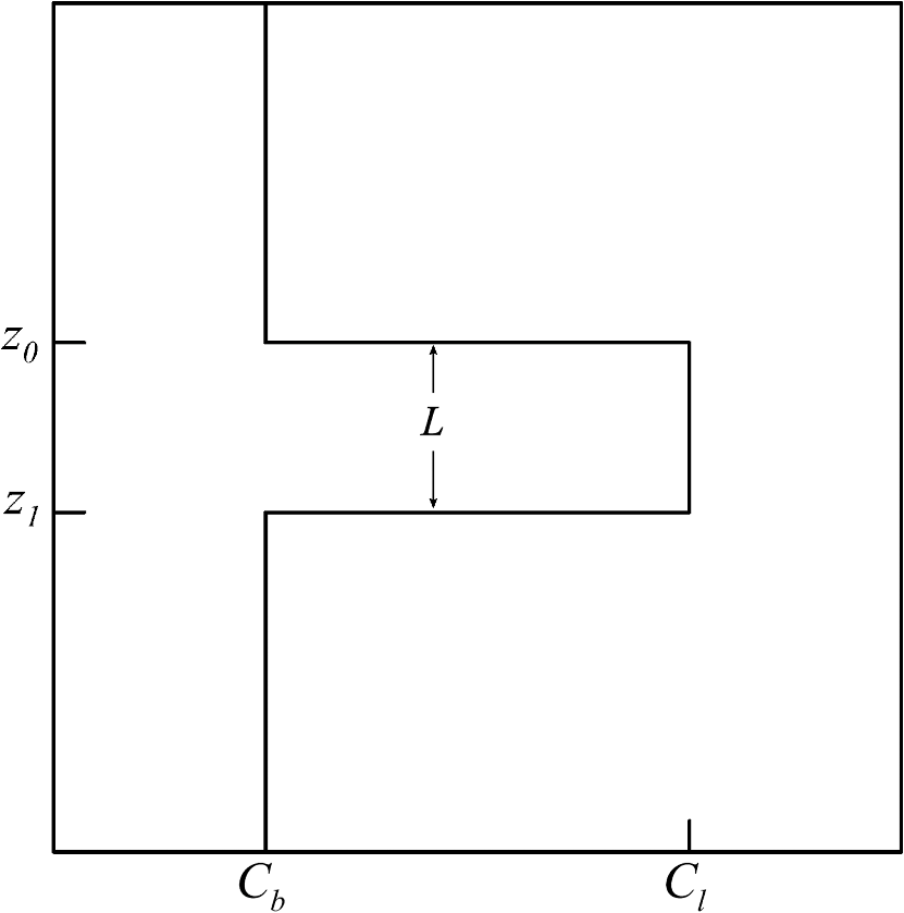$C_b$.

We considered the example of two wavelengths used in the OC3M algorithm, 443 nm in the blue and 547 nm in the green, and a 3-m thick layer whose chlorophyll concentration was 10 times the background concentration. The factor-of-ten enhancement is consistent with reported values that include a range of 4-55 in Monterey Bay, California⁵⁶ and a median value of 12 in open water in the Arctic Ocean.⁵⁷ A minimum value of three was used as a criterion for the existence of a layer in East Sound, Washington,⁴⁰ suggesting typical values were much higher. However, other measurements in Monterey Bay have produced average values of about three,^42,58 suggesting that there is a high degree of variability. Figure 6 presents the results for layers at depths (to the center of the layer) of 5 and 10 m, along with the results without a layer. The effect of the layer is most pronounced at the blue wavelength, especially at the shallower depth and at lower values of chlorophyll concentration. The effect is small at the green wavelength, where $R_{\mathrm{rs}}$ is nearly constant over a wide range of chlorophyll concentrations. The spectra of Fig. 2 illustrate that this lack of sensitivity is a consequence of the selection of 547 nm as the green wavelength.

Fig. 6

Remote sensing reflectance, $R_{\mathrm{rs}}$, as a function of background chlorophyll concentration, $C_b$, for wavelengths of 443 and 547 nm. For each wavelength, curves are plotted for no layer (solid line) and 3-m thick layers at depths of 5 m (short-dashed line) and 10 m (long-dashed line).

The shift in remote sensing reflectance will affect the inferred chlorophyll concentration. Using the same conditions of a 3-m thick layer whose concentration is 10 times the background concentration, we investigated the effects of layer depth (Fig. 7). At low-background concentrations, the concentration inferred from remote sensing reflectance is generally higher than the background concentration for shallow layers. At higher background concentrations, the layer has much less of an effect unless it is right at the surface.

Fig. 7

Estimated chlorophyll concentration, $C_{\mathrm{est}}$, as a function of background concentration, $C_b$, for the case of no layer (solid line), a 3-m layer at the surface (short dashed line), and at depths of 2.5, 5, and 10 m (dashed lines with increasing dash length).

To illustrate the effects on primary productivity, we will consider a midlatitude (45°N), midsummer (year day 180) example (Fig. 8). As the background chlorophyll concentration increases, deeper layers see less light and contribute less to the total productivity. For a layer at 40 m, the contribution from the layer goes to zero when $C_B=1\mathrm{mg}{\mathrm{m}}^{-3}$. For a layer at 20 m, this happens at $C_B=6\mathrm{mg}{\mathrm{m}}^{-3}$. The maximum productivity for this example generally occurs for a layer at 5 to 10 m deep.

Fig. 8

Calculated column-integrated primary productivity, PP, as a function of background chlorophyll concentration, $C_b$, for the case of no layer (solid line), and 3 m layers at depths of 2.5, 5, 10, 20, and 40 m (dashed lines with increasing dash length).

The comparison of calculated productivity with that estimated from satellite measurements (Fig. 9) shows that significant errors can occur when thin layers are present. For layers at depths of 5 to 10 m, productivity is underestimated by more than a factor of two. For the deepest layer, the satellite estimate is about 8% greater than the calculated value. This is a result of the approximations inherent in Eq. (24) rather than an effect of the layer.

Fig. 9

Estimated column-integrated primary productivity, ${\mathrm{PP}}_{\mathrm{est}}$, as a function of calculated productivity, PP, for 3 m thick layers at depths of 2.5, 5, 10, 20, and 40 m (dashed lines with increasing dash length). Solid line is ${\mathrm{PP}}_{\mathrm{est}}=\mathrm{PP}$.

6.

Conclusions

The remote-sensing reflectance of the ocean will be affected by the presence of thin layers of enhanced chlorophyll concentration. For case 1 waters, a bio-optical model was used to demonstrate that this effect depends on the background chlorophyll concentration, enhancement in the layer, depth of the layer, and optical wavelength. Because of the wavelength dependence, estimates of chlorophyll concentration-based ratios of remote sensing reflectance at different wavelengths will also be affected. This effect leads to estimates of primary productivity that are too low when ocean color alone is used.

Thin layers at 5–10 m depths produce the worst estimates of chlorophyll concentration and primary productivity. This is significant for productivity at midlatitudes because the seasonal thermocline that would support layers at these depths is typically shallow in spring and summer when productivity is greatest. In fact, thin layers within this depth range are common in Monterey Bay, California,⁵⁹ East Sound, Washington,⁴⁰ West Sound, Washington,⁴⁹ and elsewhere.³⁹ Deeper layers are also common, and the total column-integrated chlorophyll concentration will be underestimated where these occur. These layers receive less sunlight, however, and their contribution to total primary productivity is small.

The same bio-optical model can be used to describe the signal from a profiling lidar. With the application of a previously developed relationship between backscatter and attenuation and a new inversion technique, the lidar signal reproduces the profile of chlorophyll concentration, including the characteristics of the layer. As a result, estimates of primary productivity obtained from lidar do not exhibit the same bias inherent in those obtained from ocean color. With this model, future work will concentrate on combining active and passive sensors to improve estimates of chlorophyll concentration and primary productivity using the spectral information from passive sensors and the profile information from active sensors.