1.

Introduction

The New Zealand Land Cover Database¹ (LCDB) is a digital thematic map of land cover and land use. It is mainly produced by manual digitization using satellite imagery and aerial photographs. In the large and relatively homogenous pasture areas, small patches of woody vegetation are often not identified correctly by human interpretation. An automated, or at least a semiautomated, approach for woody/nonwoody classification using imagery that is available nation-wide would, therefore, be desirable in order to improve map quality. As the major aim of this study is to improve the information content of an existing dataset, such a method must be “conservative” in the sense that it only adds new polygons that are woody with a high probability. The improvement of manually digitized land cover maps is a problem that is not specific to the LCDB and the method could, therefore, also be applied to regional and national land cover maps in other regions of the world.

Current methods for automated land cover mapping on the regional to national scale are well established for single-source approaches using synthetic aperture radar (SAR) and optical datasets² as well as synergistic use of SAR and optical imagery that generally produces improved classification results.^3–7

A wide range of supervised classification methods are described in this literature. These include statistical methods, such as maximum likelihood and discriminant analysis, machine-learning methods, such as decision tree classifiers, neural networks, and support vector machines⁸ (SVMs). A number of studies point out that SVMs are effective in classifying high-dimensional input datasets.^9–12 Mountrakis et al.¹³ even conclude that “past applications of the method on both real-world data and simulated environments have shown that SVMs exhibit superiority over most of the alternative algorithms.” Geographic object-based image analysis provides advantages over pixel-based techniques^14–17 and is well suited to analyses that combine different data sources as image registration differences average out over segments.

The use of light detection and ranging (LiDAR)-derived canopy height models (CHMs) for forest mapping is equally well established with the promise of high spatial resolution and associated high accuracy. Classification results can be improved by combination with data from other sensors.² However, LiDAR data are rarely available as full coverage for regional and national mapping initiatives due to the high cost. Nevertheless, for small-scale mapping, it is valuable as a training data, at least if the features to be mapped can be well identified by the LiDAR-derived products.

It is surprising that despite the existence of methods for automated land cover mapping on regional to national scales, many mapping programs are still mainly created using manual digitization techniques—e.g., the LCDB of New Zealand and the “Peta Penutupan Lahan”¹⁸ of Indonesia. The two main reasons for this are (1) the general belief that manual mapping using aerial photography is able to provide better spatial accuracy than automated classification of satellite images and (2) the need for continuity of multitemporal maps. Therefore, approaches are needed which enable automated classification to improve map quality without replacing the manual methods completely. Improvement of map quality in this context refers to the addition of information content from automated methods to the manually derived maps. This approach can also be applied to mapping programs that consider introducing new data sources, e.g., if SAR data are added to a mapping approach that is purely based on optical imagery.

In this paper, we describe a segmentation-based method for automated detection and classification of so far unmapped woody patches with a minimum mapping size of 1 ha. A LiDAR CHM is used to train the classifier regarding the woody/nonwoody discrimination, while the classification of identified woody patches uses the existing LCDB (map) in the training step. The classifier makes synergetic use of Phased Array type L-band SAR (PALSAR) and Satellite Pour l’Observation de la Terre (SPOT) data in both training steps. We describe which of the data sources are most able to differentiate between woody and nonwoody vegetation.

2.

Data

3.

Methods

We used a two-step classification with a first step differentiating between woody and nonwoody and a second step classifying identified woody patches according to the existing LCDB classes.

3.1.

Identification of Woody Patches

We first segmented the SPOT imagery using an algorithm called the iterative elimination method available in the Remote Sensing and GIS Software Library.²⁴ The algorithm uses K-means clustering²⁵ for seeding and classifying pixels in a first step. Then the classified pixels are clumped into geographically uniquely labeled regions and small clumps are merged iteratively with their most similar larger neighboring segments until the minimum mapping size is reached. Segmentation was based on the red, near-infrared (NIR), and short-wave infrared (SWIR) band of both SPOT mosaics and the minimal segment size was set to 1 ha, according to the minimum mapping unit, which resulted in 277,838 segments in the Wellington region. To allow further analysis, the segments were then associated with statistics relevant to CHM, SPOT, and PALSAR imagery as well as a prerelease of New Zealand LCDB with the version 4.1. The calculated statistics are as follows:

• • Percentage of segment area covered by CHM values larger than 3, 2, 1, and 0.5 m, respectively.

• • Mean of SPOT reflectance values of the red, NIR, and SWIR bands, as well as mean normalized difference vegetation index (NDVI).

• • Mean of PALSAR HH and HV polarized backscatter (power values, not converted to dB) and the HH/HV ratio.

• • Percentage of segment area covered by the different PALSAR quality classes.

• • Percentage of segment area covered by each of the LCDB classes.

To derive training data, we used the CHM to identify the segments that are clearly woody (more than 90% covered by CHM values larger than 3 m; 58,063 segments) and those that are clearly nonwoody (less than 10% covered by CHM values larger than 0.5 m; 82,236 segments). The thresholds for defining woody areas were chosen for the following reasons. First, we wanted to have homogenous sets of segments as a training dataset; vegetation that is higher than 3 m is certainly woody in the New Zealand context and confusion with agricultural plants such as maize and vineyards as well as flax can be avoided. The second reason for the 90% threshold is that the CHM includes built-up areas. Segments greater than 1 ha are never completely covered by buildings; therefore, a coverage value larger than 90% makes sure that built-up areas are excluded. Thirdly, a temporal difference of 7 years between the LiDAR data used for training (2014) and the PALSAR data (2007) used for application of the classification model exists. To make sure that a patch of woody vegetation identified by the CHM already existed in 2007, the thresholds, therefore, have to consider regrowth. The fastest growing vegetation type in New Zealand is pine tree plantations. Pinus radiata plantations typically grow 6 to 10 m in their first 7 years on the North Island.²⁶ However, canopy closure would not typically reach 90% except in those stands planted with exceptionally high stocking density. Therefore, the 90% threshold makes sure the woody vegetation already existed at the time the PALSAR data were recorded.

Histograms of per segment mean values of SPOT red, NIR and SWIR, NDVI, PALSAR HH and HV, and the HH/HV ratio were then created to examine the power of the seven predictors to discriminate between woody and nonwoody segments (Fig. 1). The histograms show that NDVI has very little ability to differentiate between woody and nonwoody vegetation, while all other predictors indicate some degree of discrimination between the two classes, with the best separation shown by SPOT SWIR and PALSAR HV.

Fig. 1

Histograms of woody (in green) versus nonwoody (in red) segments for each of the seven predictors. $X$-axis for Satellite Pour l’Observation de la Terre (SPOT) red, near-infrared (NIR), and short-wave infrared (SWIR) bands shows reflectance values, phased array type L-band synthetic aperture radar (PALSAR) HH, and HV decibel (dB) of backscatter. $Y$-axis describes the number of segments.

Scatterplots showing the two classes in a two-dimensional feature space were then created for all combinations of the seven predictors to visually check for potential correlation and none was detected. Figure 2 displays the three histograms showing the best differentiation based on SPOT only (red versus SWIR), PALSAR only (HH versus HV), and a combination of SPOT and PALSAR (SWIR versus HV).

Fig. 2

Scatterplots of woody (green) and nonwoody (red) segments for SPOT red versus SWIR band (reflectance), HH versus HV backscatter (dB), and SWIR band (reflectance) versus HV backscatter (dB).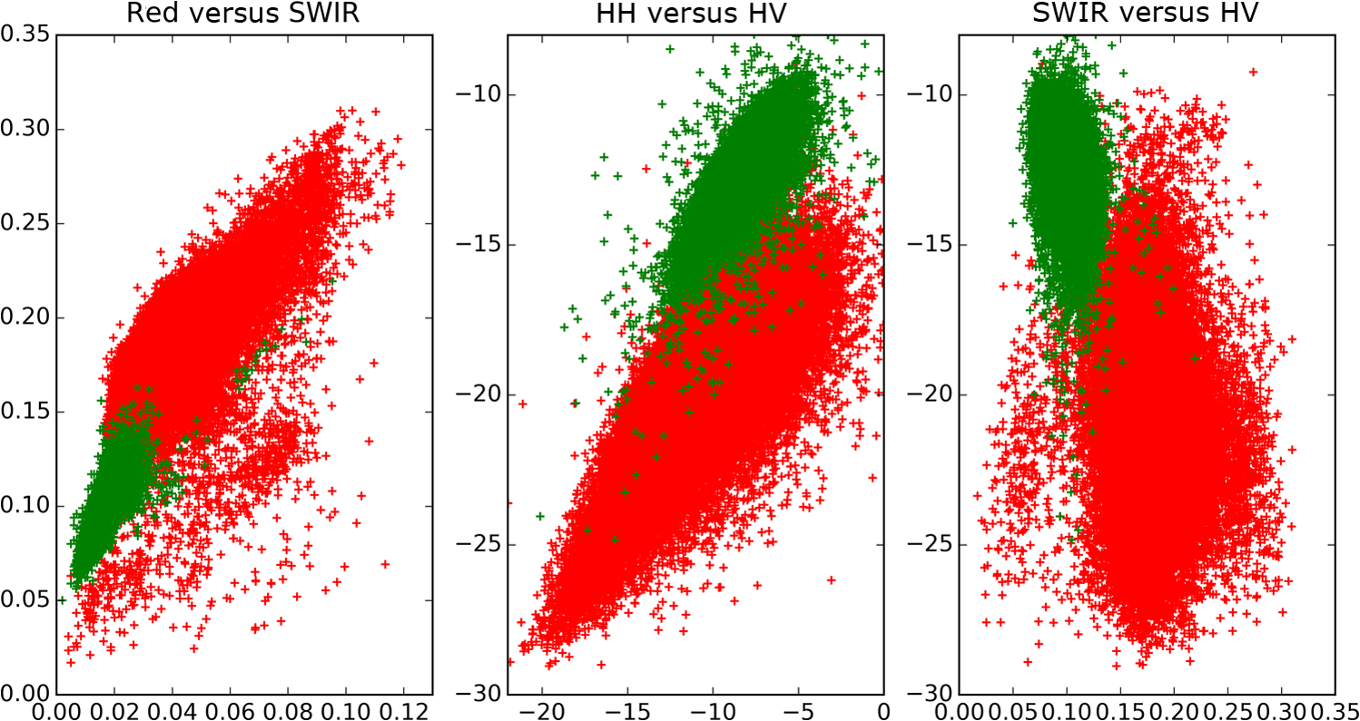

At this stage, we had identified six apparently uncorrelated predictors that had the ability to differentiate between woody and nonwoody segments with SPOT SWIR and PALSAR HV showing the best promise. We now had to find a suitable statistical model. Visual interpretation of scatterplots shows that a nonlinear differentiation function is preferable, which ruled out algorithms based on classification trees such as decision tress or random forest as well as discriminant analysis. Therefore, we decided to use SVM⁸ because of their versatility regarding the applied decision functions. Scikit-learn¹² was chosen as the corresponding software library because of the familiarity of the authors with the python programming language and its well-structured architecture and documentation.

To find the best SVM-based classifier, we compared model and cross-validation scores for different sets of predictors, different decision functions (linear, polynomial, and radial basis function), and parameterizations of the decision functions. Initial runs showed that linear as well as second- and third-degree polynomials performed best considering both physical interpretation of the discrimination function as well as model and cross-validation scores. The independent term of polynomial functions (coefficient 0) is by default set to 0 and we experimented with different values. Values of 0.05, 0.5, and 1 generally resulted in good results but performed differently for the various polynomial functions and predictor sets. Therefore, we evaluated all possible combinations of the mentioned values. The used predictor sets were as follows:

• • PALSAR only (HH and HV backscatter and HH/HV ratio);

• • SPOT only (red, NIR, and SWIR bands);

• • PALSAR HV backscatter combined with SPOT SWIR; and

• • All six predictors.

4.

Results

Comparison of the different predictor sets and kernel functions showed that it is possible to develop a classifier using any of the four parameter sets. Highest scores and cross-validation scores ($>0.99$) were achieved by the complete predictor set using third-degree polynomials and coefficient 0 set to 1.0. Scores of the SWIR/HV combination were only slightly lower. We decided to use the classifier with the overall highest score: the complete parameter set using a third-degree polynomial and a coefficient 0 of 1.0. For comparison and display purposes, we use the SWIR/HV predictor set with the same kernel parameters in parallel.

To understand how the SVM classifier differentiates between the two target classes, we created a diagram showing the discrimination function in the two-dimensional case using the SWIR/HV predictor set (Fig. 3). The third-degree polynomial calculated by the SVM algorithm separates the two classes well. As shown in Fig. 3, the brown line is the discrimination function, if the woody and nonwoody classes use a weighting of 1:10. The reason for this weighting is that we want conservative identification of new woody patches, given that our general purpose is to improve the LCDB dataset. Therefore, introduction of segments that are incorrectly identified as woody is avoided. Weighting the two classes achieves this by moving the discrimination function closer to the woody cluster reducing the number or segments identified as woody and thus reducing false positives.

Fig. 3

Plot of nonweighted (yellow/blue area) and weighted (brown line) discrimination function between woody and nonwoody classes. $X$-axis shows the SPOT SWIR band and $Y$-axis the PALSAR HV backscatter, both standardized (centered to 0 and scaled to unit variance).

The woody/nonwoody classifier was trained with segments that were homogenous (defined by the 90% larger than the 3-m CHM-value threshold). To better understand the classifier when using heterogeneous segments, we applied it to all segments thus far classified by LCDB as pasture (LCDB classes “High-Producing Exotic Grassland,” “Low-Producing Grassland,” and “Depleted Grassland”), in the Wellington region where the LiDAR CHM was available. Overall, the Wellington region was divided into 272,856 segments. Of the segments previously identified by LCDB as pasture, 4733 segments were now identified as being woody by the classifier based on SWIR and HV backscatter only, while 4880 segments were identified using the classifier based on six predictors. Figure 4 shows the newly identified woody patches (in pasture) for the Wellington region, and Fig. 5 shows a subset of this.

Fig. 4

Land Cover Database (LCDB) map of the Wellington region, showing newly identified woody patches in pasture, as red.

Fig. 5

A subset of the Wellington region (LCDB), showing newly identified woody patches outlined in red. The woody patches are classified as outlined in Sec. 3.2.

We then compared how many of the identified segments were also identified using CHM thresholds. For this, we identified those segments with a majority ($>50\%$) covered by CHM values greater than 3, 2, 1, and 0.5 m, respectively (Table 1). According to this analysis, the classifier based on six predictors performed better than the one based on SWIR and HV when applied to real-world data, which is in accordance with model and cross-validation scores. For the height class, where the majority of woody vegetation has a height greater than 0.5 m, over 92% of the segments were correctly classified as woody.

Table 1

Comparison of number of segments identified by the SVC classifier with those identified by the light detection and ranging canopy height model (LiDAR CHM).

Both steps of the classifier were then applied to all 16 regions of New Zealand. The resulting raster clumps were polygonized and smoothed. To simplify inclusion in LCDB 4.1, the polygons were then filtered using a WITHIN spatial operation with existing pasture polygons. The output of this filter operation only included isolated and completely new polygons that could easily be checked by an operator before inclusion. Table 2 shows the number of these found in each region before and after filtering. The 16,840 isolated and smoothed polygons were visually checked against a temporal sequence of older Landsat7 imagery, the SPOT-5 imagery used in this study, more recent Landsat8 imagery, and more recent high-resolution SPOTMaps imagery (1.5 m). Each of these isolated woody features was assessed to see if it would be an improvement to the LCDB if included without any additional digitizing. The proportion considered useful was 76% (12,743). Those woody features considered to be an improvement were manually classified into LCDB categories by interpretation of the temporal image sequence and directly inserted into the LCDB. The prediction of which woody class the feature fell in was less accurate, in all 4627 (7783 ha) were correctly predicted or 36%.

Table 2

Statistics for discovered woody features with potential to improve LCDB. For each region, the first figure is the total number of woody features and the second figure is the reduction after filtering to ensure the feature is isolated and completely new to LCDB4.1.

5.

Discussion

Land cover classification based on a combination of optical and SAR data depends on the capability of the input bands to discriminate between the target classes and a discrimination function that is able to take advantage of this discriminative power. Our results show that it is possible to create a successful classifier based on SPOT-5 or PALSAR dual-polarized data alone, but best results are achieved when the two data sources were combined. Model and cross-validation scores were very high ($>0.99$) in the initial classification with two output classes. In the second classification step, achieved scores were much lower. This reflects the difficulty of differentiating between the multiple target classes and the quality of the LCDB used to train the classifier.

The SVM algorithm used in this study was able to differentiate between the target classes with better results in the woody/nonwoody only case and shows general potential for analysis of combined datasets because of its flexibility regarding the applied discrimination function. Furthermore, it was helpful to be able to visualize the discrimination function, although only for two-dimensional parameter sets. This allowed compensating for one of the disadvantages of many machine-learning methods—their tendency to create black box models—and enabled us to understand and interpret the model from a physical perspective.

Although we have shown that it is possible to add new information content to the existing LCDB dataset with synergetic usage of LiDAR, SPOT, and PALSAR data, manual examination of the output is still a necessity and will be in the future. We see potential, though, in refining and extending the defined methodology for future updates of LCDB. Manual work could then be redirected from on-screen drawing to quality assurance of automatically created improvement datasets.

The developed method is applicable to other mapping projects on regional to national scales if the examined landscape is characterized by a mosaic of woody and nonwoody vegetation types. The approach used can also be applied to similar problems, e.g., the identification of clearings in woody areas. A more challenging problem that would need adjustment of the methodology would be to find segments of incorrectly identified vegetation where the discrimination is not clear-cut woody versus nonwoody. An example would be to identify forest areas on bush/scrub backgrounds. The training method of the SVM classifier using the CHM would have to be refined in this case and the temporal difference between the PALSAR and SPOT data would pose a greater problem than in this analysis. Current and temporally matching datasets for PALSAR, SPOT, and LiDAR CHM would generally be beneficial.

The ALOS satellite that produced the PALSAR data used in this study ceased to function in 2011, but fortunately ALOS-2 started regular provision of PALSAR-2²⁷ data on December 1, 2014, with improved spatial resolution. Therefore, it should be possible to repeat the analysis described here in the future with more current SAR data. SPOT-6, on the other hand, no longer provides a SWIR band,²⁸ which was found to be the most useful of the optical bands for woody/nonwoody discrimination. Therefore, the combination of PALSAR-2 and SPOT-6 might be a powerful combination for future vegetation classification, with PALSAR-2 compensating for the missing SWIR band.

6.

Conclusion

It is possible to use a LiDAR CHM of a region as training data for a classifier. The classifier is an SVM applied to nationally available PALSAR and SPOT-5 imagery. Application of the classifier to segments increased the accuracy to levels suitable for use in enhancing the national LCDB ($\sim 92\%$). Regional-scale differentiation between woody and nonwoody vegetation was best achieved by a combination of L-band dual-polarized PALSAR data (HV) with multispectral optical data that include an SWIR band. The application of an SVM algorithm to these data proved successful. The versatility of these algorithms regarding the discrimination function and their ability to solve classification problems with multiple output classes were critical factors for success. The identified and classified woody patches constitute a valuable addition and enhancement of the national LCDB.