Three-dimensional interferometric inverse synthetic aperture radar imaging of maneuvering target based on the joint cross modified Wigner-Ville distribution

Qian Lv; Tao Su; Jibin Zheng; Jiancheng Zhang

doi:10.1117/1.JRS.10.015007

28 January 2016 Three-dimensional interferometric inverse synthetic aperture radar imaging of maneuvering target based on the joint cross modified Wigner-Ville distribution

Qian Lv, Tao Su, Jibin Zheng, Jiancheng Zhang

Author Affiliations +

Journal of Applied Remote Sensing, Vol. 10, Issue 1, 015007 (January 2016). https://doi.org/10.1117/1.JRS.10.015007

Abstract

Inverse synthetic aperture radar (ISAR) can achieve high-resolution two-dimensional images of maneuvering targets. However, due to the indeterminate relative motion between radar and target, ISAR imaging does not provide the three-dimensional (3-D) position information of a target and suffers from great difficulty in target recognition. To tackle this issue, a 3-D interferometric ISAR (InISAR) imaging algorithm based on the joint cross modified Wigner-Ville distribution (MWVD) is presented to form 3-D images of maneuvering targets. First, we form two orthogonal interferometric baselines with three receiving antennas to establish an InISAR imaging system. Second, after the uniform range alignment and phase adjustment, the joint cross MWVD is used for all range cell of each antenna pair to generate the separation of the scatterer as well as preserve the phase that contains position information of the scatterer. At last, the 3-D images of the target can be directly reconstructed from the distribution. Simulation results demonstrate the validity of the proposal.

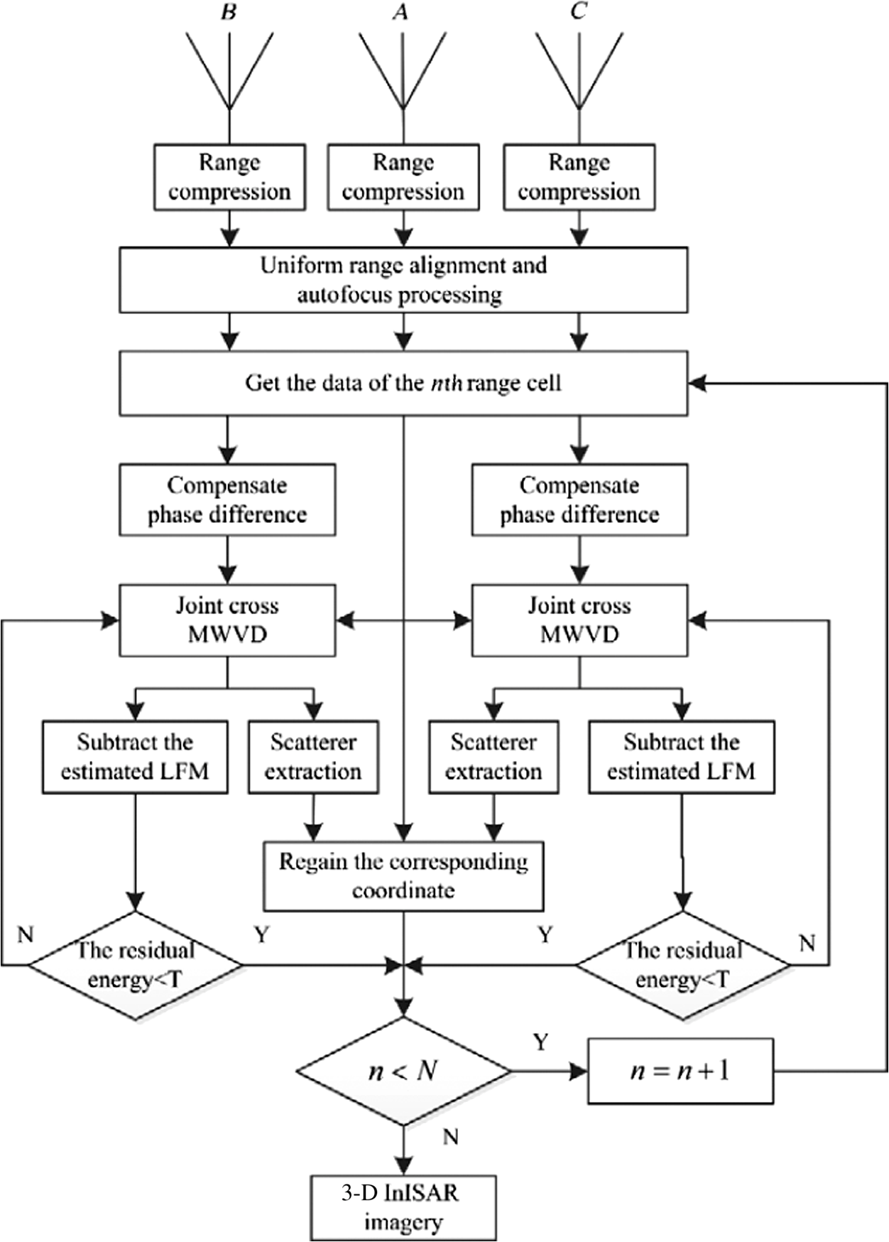
1. Introduction

Inverse synthetic aperture radar (ISAR) has been proven to be a powerful signal processing tool for imaging of moving targets in military and civilian applications.¹^–³ In ISAR imaging, the finer range resolution can be obtained by transmitting larger-bandwidth signals, while the cross-range resolution can be improved by wider aspect observations. Generally, wide aspect observations can be obtained by performing long-time observation with a monostatic ISAR or by acquiring multiaspect observations with multiple radar receiver configurations.⁴ In other words, multiaspect observations can be utilized to form a higher-resolution two-dimensional (2-D) ISAR image as well as perform three-dimensional (3-D) reconstruction of a target. Reference 4 studies the parameter estimation of ISAR imaging with multiaspect observations, which further extends the application of multiaspect observations. However, in general, the ISAR image is just a 2-D range-Doppler projection of the 3-D target’s reflectivity function onto an image plane,²^,³^,⁵^,⁶ which is mainly determined by the motion of targets with respect to the line of radar sight (LOS) and cannot be predicted. Thus the conventional 2-D ISAR image no longer meets the increasing demand of target recognition and target identification to some extent.

Recently, to further improve the ability of target recognition, especially for a noncooperative target, many algorithms are introduced for different imaging modes. Reference 7 puts forward the data level fusion method with multiaspect observations, which can obtain the target spatial structure information with known imaging geometry. In contrast to 2-D ISAR images, given the capability of providing the target’s structure information, the 3-D ISAR imaging techniques for maneuvering targets have attracted wide attention in many applications such as target identification and target recognition.⁸^,⁹ There is much literature that covers 3-D ISAR images with various algorithms. The algorithms in Refs. 10 and 11 require a 2-D antenna array to generate the 3-D images of a target; however, multiantennas inevitably result in great system complexity. References 12 13.14.15.–16 present the interferometric ISAR (InISAR) imaging technique, which combines the interferometric processing and ISAR processing to form 3-D images. Fortunately, the InISAR imaging technique has notable advantages over the aforementioned techniques in both system structure and signal processing; therefore, it attracts the attention of many researchers.

Nevertheless, in order to employ interferometry via each antenna’s ISAR images, the InISAR imaging techniques in Refs. 12 and 15 take the linear time-frequency transform and searching procedure successively, but neglect the bilinear time-frequency transform with the higher time-frequency resolution. Different from the aforementioned InISAR technique, this paper presents a 3-D InISAR imaging algorithm for maneuvering targets based on the joint cross modified Wigner-Ville distribution (MWVD). In this paper, three antennas forming two orthogonal interferometric baselines are located in the same plane orthogonal to the LOS, and a uniform range alignment and phase adjustment must be implemented together on the three antennas’ echo signals to keep the coherence among them. In addition, the joint cross MWVD of the data acquired from each two antennas located along one baseline can be adopted for each range cell, and then the 3-D structure positions of all scatterers can be solved directly from the preserved phase information in the distribution, where each scatterer is distinctly separated. Meanwhile, the 3-D images of the maneuvering target can be obtained.

The remainder of this paper is organized as follows. The InISAR system model and signal format are described in Sec. 2. In Sec. 3, the joint cross MWVD and its application are discussed in detail. Section 4 gives the analyses of the cross-terms suppression and the computational cost. In Sec. 5, a 3-D InISAR imaging algorithm is proposed based on joint cross MWVD. Finally, the simulation results of the presented algorithm and the conclusion are given in Secs. 6 and 7.

2. Interferometric Inverse Synthetic Aperture Radar Model and Signal Format

The InISAR system in Fig. 1 is based on the assumption that the model is the approximate choice for real application scenarios. The proposed model consists of three antennas located at points $A$ , $B$ , and $C$ , respectively, and $X Y Z$ defines a Cartesian coordinate with the origin $O$ as the location of the antenna $A$ . In order to achieve 3-D images of the target, these antennas have to lie on a horizontal and a vertical baseline, respectively. Antenna $A$ , doubling as both a transmitter and a receiver, is chosen at the origin; the LOS is the axis $Y$ , and the receiving antennas $B$ and $C$ are located on the axis $X$ and axis $Z$ with the coordinates $(- L, 0,0)$ and $(0,0, - L)$ , respectively.

Fig. 1

Geometry in the InISAR system.

In practical application, a maneuvering target will produce rotational motion that is represented by the rotation vector $ω_{T}$ , whose projection onto the plane perpendicular to the LOS is called the effective rotation vector $ω_{e}$ . The point $O^{'}$ is assumed to be the autofocus center for three receivers during the whole observation time, which will be mentioned in Sec. 3.

Assume the transmitted linear frequency modulation (LFM) signal takes the following form:

Eq. (1)

s (t) = \exp [j 2 π (f_{c} t + \frac{1}{2} μ t^{2})] | t | \leq \frac{T_{s}}{2},

where

t

,

T_{s}

,

f_{c}

, and

μ

denote the fast time, the pulsewidth, the carrier frequency, and the chirp rate (CR), respectively. After pulse compression, the echo signal at the receiver

Γ (A, B, C)

from the scatterer

P (x_{P}, y_{P}, z_{P})

can be represented as

Eq. (2)

s_{Γ_{P}} (t, t_{m}) = δ_{P} B \sin c {B [t - \frac{R_{A_{P}} (t_{m}) + R_{Γ_{P}} (t_{m})}{c}]} \exp [- j 2 π \frac{R_{A_{P}} (t_{m}) + R_{Γ_{P}} (t_{m})}{λ}],

where

t_{m}

is the slow time,

δ_{P}

is the amplitude,

B

is the transmitted signal bandwidth, and

λ = c / f_{c}

is the wavelength.

R_{Γ P} (t_{m})

denotes the distance of the antenna

Γ (A, B, C)

to the scatterer

P

, and this can be expressed as

Eq. (3)

R_{A_{P}} (t_{m}) = {{[x_{p} + Δ R_{x_{P}} (t_{m})]}^{2} + {[y_{p} + Δ R (t_{m}) + Δ R_{y_{P}} (t_{m})]}^{2} + {[z_{p} + Δ R_{z_{P}} (t_{m})]}^{2}}^{1 / 2},

Eq. (4)

R_{B_{P}} (t_{m}) = {{[x_{p} + L + Δ R_{x_{P}} (t_{m})]}^{2} + {[y_{p} + Δ R (t_{m}) + Δ R_{y_{P}} (t_{m})]}^{2} + {[z_{p} + Δ R_{z_{P}} (t_{m})]}^{2}}^{1 / 2} = R_{A_{P}} (t_{m}) + \frac{2 [x_{p} + Δ R_{x_{P}} (t_{m})] L + L^{2}}{2 R_{A_{P}} (t_{m})},

Eq. (5)

R_{C_{P}} (t_{m}) = {{[x_{p} + Δ R_{x_{P}} (t_{m})]}^{2} + {[y_{p} + Δ R (t_{m}) + Δ R_{y_{P}} (t_{m})]}^{2} + {[z_{p} + L + Δ R_{z_{P}} (t_{m})]}^{2}}^{1 / 2} = R_{A_{P}} (t_{m}) + \frac{2 [z_{p} + Δ R_{z_{P}} (t_{m})] L + L^{2}}{2 R_{A_{P}} (t_{m})},

where

Δ R (t_{m})

is the range translation quantity, which is the same for all scatterers on the target, and

Δ R_{x_{P}} (t_{m})

,

Δ R_{y_{P}} (t_{m})

, and

Δ R_{z_{P}} (t_{m})

are the range displacements due to rotation of the target with respect to the autofocus center

O^{'}

as shown in Fig. 1, respectively.

Obviously, it is the $R_{Γ_{P}} (t_{m})$ in Eq. (2) that results in the range migration (the translational range migration and the rotational range migration) and Doppler frequency shift (induced by the translational motion and rotational motion). Similar to the ISAR image, in order to achieve 3-D InISAR images, the motion compensation without destroying the coherence among the three receivers should be first achieved. However, notice that the terms to work for range alignment in the three receivers are different due to the existence of the second terms in Eqs. (4) and (5). Consider, under the far-field conditions, that the target size does not exceed 60 m, and the distances of the radar to target and the baseline length are no fewer than 10,000 and 1 m, respectively. Also, assume that the autofocus point is in the $X$ and $Z$ axes, and the effective range displacements $Δ R_{x_{P}} (t_{m})$ and $Δ R_{z_{P}} (t_{m})$ do not exceed 4 m; then, we have

Eq. (6)

\frac{2 [x_{p} + Δ R_{x_{P}} (t_{m})] L + L^{2}}{2 R_{A_{P}} (t_{m})} \leq \frac{2 (60 + 4) \times 1 + 100}{2 \times 10,000} \leq 0.05 m,

Eq. (7)

\frac{2 [z_{p} + Δ R_{z_{P}} (t_{m})] L + L^{2}}{2 R_{A_{P}} (t_{m})} \leq \frac{2 (60 + 4) \times 1 + 100}{2 \times 10,000} \leq 0.05 m .

The distance differences induced by rotation between three antennas are much smaller than the range resolution, when the radar range resolution is 0.1 to 0.3 m. Therefore, under this approximation, the translational range migration of all three receivers can be accomplished by using the same range alignment compensation function. Here we choose receiver $A$ as the reference channel to implement the translational range migration and the Doppler frequency shift induced by the translation, which are the same for all scatterers on the target and can be eliminated by the standard range alignment method¹⁷^,¹⁸ and the phase gradient autofocus method,¹⁹ respectively.

However, when the target size is a little larger and the required resolution becomes higher, the migration through resolution cells (MTRC), which is related to the location of each scatterer, can no longer be neglected. The Radon–Fourier transform and generalized Radon–Fourier transform (RFT/GRFT) were proposed in Refs. 20 21.–22 to deal with the couple between the envelope and Doppler, which has been shown to be very effective in muchliterature.²⁰^–²³ Thus, the RFT can be used to mitigate the MTRCs and correct all scatterers into the right cell. We will not make a detailed discussion about range alignment in this paper and will only focus on the Doppler frequency shift induced by rotational motion for 3-D InISAR reconstruction.

After the motion compensation, the azimuth echo from the scatterer $P$ can be rewritten as

Eq. (8)

s_{Γ_{P}} (t_{m}) = σ_{P} \exp [- j Φ_{Γ_{P}} (t_{m})] = σ_{P} \exp [- j 2 π \frac{R_{A_{P}} (t_{m}) + R_{Γ_{P}} (t_{m})}{λ}],

where

σ_{P}

is the relative amplitude. For simplicity, the exponential term in Eq. (8) can be further expressed as follows; and the detailed derivation is given in the Appendix.

Eq. (9)

s_{Γ_{P}} (t_{m}) = σ_{P} \exp (- j ϕ_{Γ_{P}}) \exp [- j \frac{4 π}{λ} Δ R_{y_{P}} (t_{m})],

where

Eq. (10)

ϕ_{A_{P}} = \frac{4 π}{λ} R_{P}, ϕ_{B_{P}} = \frac{4 π}{λ} R_{P} + \frac{2 π L x_{p}}{λ R_{P}}, ϕ_{C_{P}} = \frac{4 π}{λ} R_{P} + \frac{2 π L z_{p}}{λ R_{P}} .

From Eq. (10), although the terms $ϕ_{Γ_{P}}$ are independent of the slow time and unnecessary for the ISAR imaging, they carry significant position information of the scatterer, which should be preserved in the 3-D InISAR image processing, the details of which will be thoroughly explained in Sec. 3.2. The second terms in Eq. (9), completely consistent with each other in three antennas, can work for separating the different scatterers in the same range cell. From Eqs. (9) and (10), we obtain

Eq. (11)

Δ ϕ_{A B} = ϕ_{B_{P}} - ϕ_{A_{P}} = \frac{2 π L x_{p}}{λ R_{P}}, Δ ϕ_{A C} = ϕ_{C_{P}} - ϕ_{A_{P}} = \frac{2 π L z_{p}}{λ R_{P}} .

Combined with the range information $R_{n} \approx R_{P}$ , where $R_{n}$ is the distance of the radar to the $n$ ’th range cell, the position of the scatterer $P$ can be obtained as

Eq. (12)

x_{p} = \frac{λ R_{n} Δ ϕ_{A B}}{2 π L}, y_{P} = R_{n}, z_{p} = \frac{λ R_{n} Δ ϕ_{A C}}{2 π L} .

Therefore, the interferometric phase information is crucial to successfully reconstruct the 3-D position of target, which is also the research emphasis in this paper.

3. Joint Cross Modified Wigner-Ville Distribution

3.1.

Proposed Algorithm for Signal Separation

After the uniform motion compensation, the position of the autofocus centers for each ISAR image remains the same relative to the three receiving antennas during the imaging time. Identical to the ISAR image for maneuvering targets, the effective rotating velocities $ω_{x}$ and $ω_{z}$ are time-variant and do cause the change of the Doppler frequency, which can be utilized to realize the high-resolution ISAR imaging. They can be approximated as

Eq. (13)

ω_{x} (t_{m}) = α_{x} + β_{x} t_{m}, ω_{z} (t_{m}) = α_{z} + β_{z} t_{m} .

Thus, the corresponding effective range displacement can be expressed as

Eq. (14)

Δ R_{y_{P}} (t_{m}) = x_{P} \int_{0}^{t_{m}} ω_{x} (μ) d μ + z_{P} \int_{0}^{t_{m}} ω_{z} (μ) d μ = x_{P} (α_{x} t_{m} + \frac{1}{2} β_{x} t_{m}^{2}) + z_{P} (α_{z} t_{m} + \frac{1}{2} β_{z} t_{m}^{2}) .

Then the echo signals received by receivers $A$ , $B$ , and $C$ in the $n$ ’th range cell become, respectively,

Eq. (15)

s_{Γ} (t_{m}) = \sum_{i}^{P} σ_{i} \exp (- j ϕ_{Γ_{ι}}) \exp [j 2 π (f_{i} t_{m} + \frac{1}{2} μ_{i} t_{m}^{2})],

where

f_{i} = - 2 (x_{i} α_{x} + z_{i} α_{z}) / λ

and

μ_{i} = - 2 (x_{i} β_{x} + z_{i} β_{z}) / λ

denote the centroid frequency (CF) and the CR of the

i

’th scatterer, respectively. It can be found from Eq. (15) that the echo signals received by the three antennas have the LFM signal format. Therefore, they can be solved by the same processing algorithms as the LFM signal, such as WVD,²⁴ which is extensively applied for ISAR imaging. However, when the WVD is directly used on the echo signal itself of a single antenna, the interferometric phases will be completely lost. As a result, the joint cross MWVD is introduced to separate the scatterer in the same range cell due to its good phase preservation and searching-free procedure, where the term “joint cross” refers to the joint cross-correlation operation of the data acquired from two different antennas of all three antennas. The key to the so-called joint cross MWVD in this paper is the definition of the symmetric instantaneous cross-correlation function (SICCF) from the two different receivers, which is essentially different from the MWVD that performs the instantaneous autocorrelation only aiming at one receiver. The results of bilinear transform on the signal itself in Ref. 24 will bring about the loss of the time-invariant interferometric phase information, which further results in the failure in the image interferometry. Given the symmetric relation of the antennas

B

and

C

, here we only take the interferometric antenna pair

A B

as an example to explain the above analysis. The SICCF of the receiver pair

A B

can be defined by

Eq. (16)

R_{A B} (t_{m}, τ) = s_{A} (t_{m} + \frac{τ}{2}) s_{B}^{*} (t_{m} - \frac{τ}{2}) = \sum_{i}^{P} σ_{i}^{2} \exp (j Δ ϕ_{A B}) \exp [j 2 π (f_{i} + μ_{i} t_{m}) τ] + R_{A B, cross},

where

s_{A} (t_{m})

and

s_{B} (t_{m})

denote the echo signals received by receivers

A

and

B

in the

n

’th range cell, respectively.

τ

is the lag variable, and

R_{A B, cross}

denotes the cross-terms. By performing the normal WVD transform on Eq. (16), we have

Eq. (17)

W_{A B} (t_{m}, f_{τ}) = \int s_{A} (t_{m} + \frac{τ}{2}) s_{B}^{*} (t_{m} - \frac{τ}{2}) \exp (- j 2 π f_{τ} τ) d τ = \sum_{i}^{P} σ_{i}^{2} \exp (j Δ ϕ_{A B}) δ [f_{τ} - (f_{i} + μ_{i} t_{m})] + W_{A B, cross} .

In Eq. (17), the slow time variable $t_{m}$ and the lag variable $τ$ linearly couple with each other; thus, the joint cross WVD between the receiver pairs $A B$ peaks along the straight line $f_{τ} = f_{i} + μ_{i} t_{m}$ , whose intercept and slope are related to the CF $f_{i}$ and the CR $μ_{i}$ of the $i$ ’th scatterer. Borrowing the idea from the classical scale transform (ST), we propose the joint cross MWVD, which can be denoted as

Eq. (18)

G_{A B} (f_{τ}, f_{τ t_{m}}) = \iint_{τ, τ t_{m}} R_{A B} (t_{m}, τ) d [τ t_{m}] d [τ] = \sum_{i}^{P} σ_{i}^{2} \exp (j Δ ϕ_{A B}) δ (f_{τ} - f_{i}) δ (f_{τ t_{m}} - μ_{i}) + G_{A B, cross},

where

G_{A B, cross}

are the cross-terms corresponding to the MWVD, which will be discussed later.

For Eq. (18), the linear couple between the slow time variable $t_{m}$ and the lag variable $τ$ is removed, and the signal energy is completely accumulated only by FFT operation without searching any parameters. Also, it is clearly seen that the CF and the CR are closely related to its coordinates; different scatterers with different coordinates will be discriminated from each other in the centroid frequency and chirp rate domain (CFCRD). After the joint cross MWVD, each scatterer can be easily separated as a peak point in the CFCRD.

3.2.

Proposed Algorithm for Information Extraction

Without loss of generality, the joint cross MWVD of the scatterer $P$ from the antenna pair $A B$ can be denoted as

Eq. (19)

G_{A B} (f_{τ}, f_{τ t_{m}}) = {FFT}_{τ} ({FFT}_{t_{m}^{'}} {{ST}_{τ t_{m}} [R_{A B} (t_{m}, τ)]}) = σ_{p}^{2} \exp (j Δ ϕ_{A B}) δ (f_{τ} - f_{p}) δ (f_{τ t_{m}} - μ_{p}),

where

t_{m}^{'}

denotes the new time variable after ST.

G_{A B} (f_{τ}, f_{τ t_{m}})

has a sole peak at the point

(f_{p}, μ_{p})

and can be modeled as an ideal point spread function. Also, more attention should be paid to the face that the interferometric phase information

Δ ϕ_{A B}

of each scatterer is well preserved in Eq. (19) then the phase differences can be computed as follows:

Eq. (20)

Δ ϕ_{A B} = ∠ [G_{A B} (f_{p}, μ_{p})], Δ ϕ_{A C} = ∠ [G_{A C} (f_{p}, μ_{p})] .

We can use Eq. (12) to solve the 3-D position of all scatterers in the n’th range cell. Hence, the 3-D positions of all scatterers on the target will be easily obtained by using the same process in all range cells.

In addition, it is also worthwhile to mention that only when the phase differences $Δ ϕ_{A B}$ and $Δ ϕ_{A C}$ do not exceed $2 π$ is the solution to $(x_{p}, z_{p})$ in Eq. (12) correct. Hence,

Eq. (21)

Δ ϕ_{A B} = \frac{2 π L x_{p}}{λ R_{P}} \leq 2 π, Δ ϕ_{A C} = \frac{2 π L z_{p}}{λ R_{P}} \leq 2 π

must be satisfied. Note that

(x_{p}, z_{p})

depends on the aircraft size. In other words, as long as the aircraft size does not exceed

λ R_{n} / L

, the solution to

(x_{p}, z_{p})

is correct. Similar to the aforementioned consideration, the target size does not exceed 60 m, and the distance of the radar to target and the baseline length are no less than 10,000 and 1 m, respectively. Thus,

Eq. (22)

x_{p}, z_{p} \leq \frac{λ R_{n}}{L} = \frac{0.03 \times 10,000}{1} = 300 m

can always be satisfied.

3.3.

Rotation Parameter Retrieval

The rotation parameter estimation is an essential task for ISAR and has drawn much attention.²⁵^,²⁶ According to Eqs. (13)–(15), when the coordinates of the scatterer are fixed, the CF $f_{p}$ and the CR $μ_{p}$ of the scatterer $P$ mainly depend on the angular velocity $α_{x}$ , $α_{z}$ and angular acceleration $β_{x}$ , $β_{z}$ along the $X$ and $Z$ axes, respectively. That is,

Eq. (23)

f_{p} = - 2 (x_{P} α_{x} + z_{P} α_{z}) / λ = - 2 α_{e} (x_{P} \cos θ + z_{P} \sin θ) / λ,

Eq. (24)

μ_{p} = - 2 (x_{P} β_{x} + z_{P} β_{z}) / λ = - 2 β_{e} (x_{P} \cos θ + z_{P} \sin θ) / λ,

where

x_{P}

and

z_{P}

denote the coordinates of the scatterer

P

, and

α_{e}

and

β_{e}

are the effective initial rotating velocity (IRV) and effective rotating acceleration (RA), respectively.

Accordingly, the parameters $α_{e}$ and $β_{e}$ can be estimated with the estimated parameters $x_{P}$ and $z_{P}$ . We can rewrite Eqs. (23) and (24) by considering only the contribution of the $i$ ’th scatterer.

Eq. (25)

C_{i} = a X_{i} + b Z_{i},

Eq. (26)

D_{i} = c X_{i} + d Z_{i},

where

C = - λ f_{i} / 2

,

D = - λ μ_{i} / 2

,

X_{i} = x_{i}

,

Z_{i} = z_{i}

,

a = α_{e} \cos θ

,

b = α_{e} \sin θ

,

c = β_{e} \cos θ

, and

d = β_{e} \sin θ

.

C_{i}

and

D_{i}

, respectively, represent the CF and the CR of the

i

’th scatterer, which have been extracted in Eq. (19). Also, the coordinates

X_{i}

,

Z_{i}

of the

i

’th scatterer can be calculated from Eq. (12). Then, the parameters

α_{e}

and

β_{e}

can be accomplished by estimating

a

and

b

.

The situation can be mathematically dealt with by minimizing the function

Eq. (27)

Ψ (a, b) = \sum_{i}^{N_{P}} {[C_{i} - (a X_{i} + b Z_{i})]}^{2}, ϒ (c, d) = \sum_{i}^{N_{P}} {[D_{i} - (c X_{i} + d Z_{i})]}^{2},

where

N_{P}

is the number of extracted scatterers.

Consequently, the effective IRV, $α_{e}$ , and effective RA, $β_{e}$ , can be obtained by the estimated $\hat{a}$ , $\hat{b}$ , $\hat{c}$ , $\hat{d}$ .

Eq. (28)

{\hat{α}}_{e} = \sqrt{{\hat{a}}^{2} + {\hat{b}}^{2}}, {\hat{β}}_{e} = \sqrt{{\hat{c}}^{2} + {\hat{d}}^{2}} .

4. Performance of Joint Cross Modified Wigner-Ville Distribution

4.1.

Analysis of the Cross-Terms

In order to obtain the high-resolution imaging, the echo signals have to be modeled as multicomponent LFM signals in each range cell. Moreover, due to the nonlinear characteristic of the SICCF, the cross-terms are inevitable and may affect the detection of self-terms. We need to analyze the performance of the joint cross MWVD under the situation of multi-LFM signals. Here, assume that there are two scatterers, and the proof process of the multi-LFM signals can refer to the following discussion:

Eq. (29)

s_{A} (t_{m}) = s_{A_{P}} (t_{m}) + s_{A_{Q}} (t_{m}) = σ_{p} \exp (- j ϕ_{A_{p}}) \exp [j 2 π (f_{p} t_{m} + \frac{1}{2} μ_{p} t_{m}^{2})] + σ_{q} \exp (- j ϕ_{A_{q}}) \exp [j 2 π (f_{q} t_{m} + \frac{1}{2} μ_{q} t_{m}^{2})],

Eq. (30)

s_{B} (t_{m}) = s_{B_{P}} (t_{m}) + s_{B_{Q}} (t_{m}) = σ_{p} \exp (- j ϕ_{B_{p}}) \exp [j 2 π (f_{p} t_{m} + \frac{1}{2} μ_{p} t_{m}^{2})] + σ_{q} \exp (- j ϕ_{B_{q}}) \exp [j 2 π (f_{q} t_{m} + \frac{1}{2} μ_{q} t_{m}^{2})] .

After performing the SICCF on Eq. (16), we obtain

Eq. (31)

R_{A B} (t_{m}, τ) = R_{A B_{p, self}} (t_{m}, τ) + R_{A B_{q, self}} (t_{m}, τ) + R_{A B_{p q, cross}} (t_{m}, τ) + R_{A B_{q p, cross}} (t_{m}, τ),

where

Eq. (32)

R_{A B_{p q, cross}} (t_{m}, τ) = σ_{p} σ_{q} \exp [j (ϕ_{B_{q}} - ϕ_{A_{p}})] \exp {j 2 π [(f_{p} - f_{q}) t_{m} + (f_{p} + f_{q}) \frac{τ}{2} + \frac{1}{2} (μ_{p} - μ_{q}) t_{m}^{2} + \frac{1}{2} (μ_{p} + μ_{q}) τ t_{m} + \frac{1}{2} (μ_{p} - μ_{q}) \frac{τ^{2}}{4}]},

and the cross-term

R_{A B_{q p, cross}} (t_{m}, τ)

is the same as

R_{A B_{p q, cross}} (t_{m}, τ)

in essence; thus, we only take

R_{A B_{q p, cross}} (t_{m}, τ)

as an example to analyze. Then, after ST, we have

Eq. (33)

{ST}_{A B_{p q, cross}} (t_{m}^{'}, τ) = σ_{p} σ_{q} \exp [j (ϕ_{B_{q}} - ϕ_{A_{p}})] \exp {j 2 π [(f_{p} - f_{q}) \frac{t_{m}^{'}}{τ} + (f_{p} + f_{q}) \frac{τ}{2} + \frac{1}{2} (μ_{p} - μ_{q}) {(\frac{t_{m}^{'}}{τ})}^{2} + \frac{1}{2} (μ_{p} + μ_{q}) t_{m}^{'} + \frac{1}{2} (μ_{p} - μ_{q}) \frac{τ^{2}}{4}]} .

It can be found from Eq. (33) that the ST can only correct the linear CR migration of self-terms, but not of the cross-terms. Thus, the energy of self-terms is well accumulated after MWVD, while the energy of cross-terms is typically dispersed in the whole distribution. Here, we do a simulation to testify that the proposed algorithm in the paper can handle the situation of multicomponents. Consider three components denoted by AU1, AU2, and AU3, respectively. The sample frequency is 256 Hz, and the effective signal length is 512. The CF and CR of AU1, AU2, and AU3 are as follows: $f_{1} = 20 H z$ , $μ_{1} = 20 H z / s$ , $f_{2} = - 20 H z$ , $μ_{2} = 20 H z / s$ , and $f_{3} = 20 H z$ , $μ_{3} = - 20 H z / s$ .

As illustrated in Fig. 2, the couplings of the self-terms are removed by ST, but this does not work for the cross-terms. Therefore, the energy of self-terms is well accumulated in CFCRD, and the proposed method is more suitable for the complicated situation. In the above simulation, the amplitudes of the three LFM signals are considered to be the same. However, under the situation of the different amplitudes in a real-world application, the modified clean technique has to be performed to separate strong and weak LFM signals without the loss of significant interferometric phase information.

Fig. 2

Simulation results: (a) contour of WVD, (b) results after ST, (c) contour of MWVD, and (d) stereogram of MWVD.

4.2.

Analysis of the Computational Cost

Due to the existence of CR in Eq. (15), the echo signals received by the different receivers cannot be directly integrated to form the image. Therefore, algorithms have been proposed to estimate the parameter to reconstruct the 3-D position of moving target, such as Radon transform,¹⁵ chirplet decomposition algorithm,¹² and Lv’s distribution.²⁷ However, searching procedures are necessary for Radon transform and the adaptive chirplet algorithm, which will reduce the computational efficiency. Although Lv’s distribution can effectively avoid searching procedures, this advantage is at the cost of the redundancy information. However, there is little difficulty in obtaining the redundancy information to some extent due to the target’s maneuverability in real ISAR applications.²⁸

From the above key analysis, we can see that the computation is mainly decided by the part of signal separation. Therefore, the implementation procedures include the defined SICCF of each receiver pair $[O (N_{t_{m}}^{2})]$ , ST based on the chirp-z transform $[O (3 N_{t_{m}}^{2} \log_{2} N_{t_{m}})]$ , and the Fourier transform with respect to the lag variable $[O (N_{t_{m}}^{2} \log_{2} N_{t_{m}})]$ . However, the algorithms like the Radon transform and chirplet algorithm are searching techniques to find the most matched signal in the parameter domain. Because of the high computational load, $[O (M N_{t_{m}} \log_{2} N_{t_{m}})]$ , where $M$ denotes the number of searching points, which is normally greater than the number of echoes $N_{t_{m}}$ , these existing algorithms are less suitable for real-time high-resolution ISAR imaging.²⁸ Moreover, when the estimated parameters are in the larger scope, the searching steps and initial parameters’ set are more difficult to control and cannot achieve a balance.

As is well known, the RFT/GRFT (Refs. 20 21.22.–23) have been developed for motion estimation of maneuvering targets with arbitrary parameterized motion, and much research has verified the effectiveness of RFT and GRFT. What is more, GRFT have been successfully extended to space-time RFT (Ref. 29) for wideband digital array radar and 3-D space RFT (3-D SRFT)³⁰ to realize the 3-D reconstruction of the moving target. However, the research on the fast implementation for GRFT should be further conducted because of the prohibitive computational burden induced by the multidimensional searching. Fortunately, the particle swarm optimizer²⁸^,³¹ has been widely employed in solving the multiparameter searching problems mentioned above.

Nonetheless, compared to the proposed method in this paper, the 3-D SRFT in Ref. 28, where the acceleration is omitted, just aims at a slow maneuvering target via searching the minimum 3-D image entropy versus six-dimensional motion parameters. Also, the searching procedures will be more complicated with an increase of the motion parameters in many scenarios, like targets with complex motion whose rotational motion may cause quadratic phase terms.

5. Three-Dimensional Interferometric Inverse Synthetic Aperture Radar Imaging Algorithm Based on Joint Cross Modified Wigner-Ville Distribution

For 3-D InISAR imaging for maneuvering targets, the echo signals in a range cell at all receivers can be characterized as the same multicomponent LFM signals after uniform range alignment and phase adjustment. By using the MWVD algorithm without a searching procedure, the scatterer separation and phase extraction are simultaneously accomplished, and then 3-D images are achieved. Consequently, the 3-D InISAR imaging algorithm based on MWVD is illustrated in detail in the following, and the corresponding flowchart is shown in Fig. 3.

Step 1: Complete the range compression of the echo signals received by the three antennas.
Step 2: Choose antenna $A$ as the reference channel to accomplish uniform motion compensation with the existing methods in Refs. 17 18.–19, and then the scatterers on the target remain the uniform position and autofocus center for the three antennas.
Step 3: Utilize the function $\exp (j π L^{2} / λ R_{P})$ to compensate the phase difference due to $L$ .
Step 4: For each range cell, separate each scatterer in CFCRD after joint cross MWVD between two antenna pairs $A B$ and $A C$ .
Step 5: Apply the dechirping method to estimate the amplitude and subtract the estimated LFM from the original signal without loss of significant interferometric phase information. Meanwhile, extract the interferometric phase of the scatterer and regain the corresponding coordinate by using Eq. (12).
Step 6: Repeat steps 4 and 5 until the residual energy of the signal is smaller than threshold T.
Step 7: Repeat the aforementioned steps (4 to 6) until all the range cells have been finished.
Step 8: Combine the range information along the $Y$ axis and output 3-D images.

Fig. 3

Flowchart of the proposed InISAR imaging algorithm.

6. Simulation Results

In realistic applications, the scatterers on the target may be composed of some disturbed sources, and it is also possible that some scatterers may be sheltered by the body of the target. In this case, the readers can refer to Ref. 32 for a detailed solution. However, when compared to the radar wavelength, the target size is much larger; the assumption is normally valid that the scatterers on a real target can be regarded as separated point-like,⁸^,⁹^,¹²^–¹⁶ and the obtained image may be depicted by the location of strong scatterers. Therefore, the simulation in this paper is always under the condition that the scatterers on the target are point-like.

6.1.

Example A

In this section, a simple turntable target shown in Fig. 4(a) is modeled as seven scatterers. The parameters used are set as follows: target distance $R = 10 km$ , baseline length $L = 1 m$ , effective velocity $α_{x} = 0.08 rad / s$ , $α_{z} = 0.04 rad / s$ , and effective acceleration $β_{x} = 0.06 rad / s^{2}$ , $β_{z} = 0.06 rad / s^{2}$ . The pulse repetition frequency is 256 Hz, and the number of effective pulses is 512.

Fig. 4

Simulation results: (a) Ideal scatterer model, (b) the WVD of antenna $A B$ , (c) the MWVD of antenna $A B$ , and (d) 3-D reconstructed scatterer.

Figure 4(a) shows the ideal target model including seven ideal scatterer points. As is clearly seen in Fig. 4(b), in the joint cross WVD of antenna pairs $A B$ in a certain range cell (225 range cell), though the three scatterers are presented as different lines, the signal energy is not accumulated well and cross-terms do exist and should be considered in extreme cases. Based on the aforementioned consideration, we introduce the joint cross MWVD to accomplish energy accumulation without loss of the interferometric phase information. In Fig. 4(c), each scatterer is distinctly separated in the CFCRD, and the coordinates of each scatterer can be obtained easily from the interferometric phase information on its peak. Consequently, the 3-D images of a target are achieved based on the proposed joint cross MWVD algorithm. Figure 4(d) shows the reconstructed result of a 3-D InISAR image of an ideal model, where the real scatterer points are presented to make a comparison.

To quantitatively evaluate the performance of the proposed algorithm, the relative mean square error (MSE) of 3-D reconstructed coordinates is computed, and the MSE is defined by³³

Eq. (34)

MSE = \frac{{‖ R_{est} - R ‖}_{2}}{{‖ R ‖}_{2}},

where

R

and

R_{est}

represent the original data and the reconstructed data obtained by the proposed algorithm in this paper. The MSEs of the 3-D reconstructed coordinates obtained by using the proposed method are shown in Table 1.

Table 1

Reconstruction performance of example A.

Reconstructed coordinates	X-coordinate	Z-coordinate
MSE (%)	7.31	9.53

6.2.

Example B

In this simulation, we perform the proposed 3-D InISAR algorithm on a synthetic airplane model, which is a rigid object composed of 137 ideal scatterers. The corresponding parameters used are shown in Table 2 and the target in the simulation is moving along a straight line with respect to the radar LOS. Here, we assume that uniform motion compensation has been completed and all scatterers have the same autofocus center for the three antennas.

Table 2

Simulation parameters.

Radar		Target
Carrier frequency	10 G	Target distance	100 km
Bandwidth	500 M	Baseline length	10 m
pulse repetition frequency	512	Effective rotating	$X$ axis	$Y$ axis
Effective echo	1024	Velocity ( $rad / s$ )	0.12	0.40
Sample frequency	1 G	Acceleration ( ${rad / s}^{2}$ )	0.08	0.36

The models are shown in Fig. 5, and the results of the 3-D InISAR image in different views from three visual angles are given in Fig. 6, where the reconstructed results correspond to its projections on the $X Y$ , $X Z$ , and $Y Z$ planes, respectively. As is clearly seen from those figures, though not all of the scatterer are achieved correctly, the proposed algorithm can perform high-quality 3-D InISAR imaging of the maneuvering target. The position error of the scatterer shown in Fig. 6 results from the above approximation, noise, and cross-terms in the correlation algorithm. For the interference of the noise and cross-terms, the spurious scatterers have been reconstructed, which will lead to inconsistency in the number between the ideal scatterers and the reconstructed scatterers. In addition, in real ISAR imaging applications, because the number of scatterers on the target is usually unknown, the MSE of 3-D reconstructed coordinates cannot be obtained. Fortunately, the reconstruction accuracy is closely related to the parameter estimation precision.

Fig. 5

Target model.

Fig. 6

Target’s 3-D imaging result using the proposal.

Therefore, similar to providing a quantitative evaluation for the reconstruction performance of the 3-D target in Sec. 6.1, in order to characterize the parameter estimation precision of the proposed algorithm quantitatively, the MSEs of IRV and RA are calculated by using Eq. (34). Here, the input signal-to-noise is 20 dB, and the experiment is repeated 50 trials. From Table 3, it can be found that the MSEs of the estimated parameters with the proposed algorithm in the paper are relatively small and within the acceptable range in a real application scenario,³³ which indirectly demonstrates the effectiveness of the reconstruction via the joint cross MWVD algorithm. On the other hand, in order to improve the 3-D image quality in the future, more attention should be paid to the areas that can acquire a higher antinoise performance and effectively suppress cross-terms.

Table 3

Reconstruction performance of example B.

Estimated parameters	True value	Average estimated value	MSE (%)
IRV	0.4176	0.3570	14.52
RA	0.3688	0.3489	5.41

7. Conclusion

This paper has presented a 3-D InISAR imaging algorithm for maneuvering targets based on the joint cross MWVD. The characteristics of such a 3-D InISAR imaging algorithm include the following: (1) it is a nonsearching method in both cross-range resolution and interferometric phase extraction; (2) it can deal with the multicomponents due to its good performance in suppressing the cross-terms via coherent integration; and (3) it can accurately implement the retrieval of the rotation parameters, which is essential for target recognition and target identification in ISAR imaging application.

Appendices

Appendix:

Derivation of Signal Phase

This appendix mainly presents the simplification of the phase in Eq. (9). Rearranging Eqs. (3)–(5), we have

Eq. (35)

R_{A_{P}} (t_{m}) \approx R_{P} + \frac{2 y_{p} Δ R_{y_{P}} (t_{m})}{2 R_{P}} + \frac{+ 2 y_{p} Δ R (t_{m}) + {[Δ R (t_{m})]}^{2}}{2 R_{P}} \frac{+ 2 x_{p} Δ R_{x_{P}} (t_{m}) + 2 z_{p} Δ R_{z_{P}} (t_{m}) + {[Δ R_{x_{P}} (t_{m})]}^{2} + {[Δ R_{y_{P}} (t_{m})]}^{2} + {[Δ R_{z_{P}} (t_{m})]}^{2} + 2 Δ R_{y_{P}} (t_{m}) Δ R (t_{m})}{2 R_{P}},

where

R_{P} = \sqrt{x_{p}^{2} + y_{p}^{2} + z_{p}^{2}}

is the distance of the radar to scatter

P

. It is worth noting that this paper is under the assumption of far-field conditions, that is, the distance of the scatterer to the three antennas is same and is much larger than the target size. So the approximations

y_{p} \approx R_{P}

and

R_{P} ≫ x_{P}

or

z_{P}

hold. According to Eq. (35), the phase of the echo signal from the scattering center located at scatterer

P

on the target will have the form

Eq. (36)

Φ_{A_{P}} (t_{m}) \approx \frac{4 π}{λ} [R_{P} + Δ R_{y_{P}} (t_{m})] + \frac{2 π}{λ} {2 Δ R (t_{m}) + \frac{{[Δ R (t_{m})]}^{2}}{R_{O^{'}}}} + \frac{2 π}{λ} {\frac{2 x_{p} Δ R_{x_{P}} (t_{m}) + 2 z_{p} Δ R_{z_{P}} (t_{m}) + {[Δ R_{x_{P}} (t_{m})]}^{2} + {[Δ R_{y_{P}} (t_{m})]}^{2} + {[Δ R_{z_{P}} (t_{m})]}^{2} + 2 Δ R_{y_{P}} (t_{m}) Δ R (t_{m})}{R_{P}}} .

Evidently, the second terms in Eq. (36), independent of the scatterer, are just autofocus, which should be estimated and removed from all scatterers on the target in the motion compensation. Moreover, the rotation angle is small, and as demonstrated in Ref. 12, the third terms in Eq. (36) can be neglected.

After the autofocus and the aforementioned approximation, the phase in Eq. (9) can be rewritten as

Eq. (37)

Φ_{A_{P}} (t_{m}) = \frac{4 π}{λ} R_{P} + \frac{4 π}{λ} Δ R_{y_{P}} (t_{m}),

Eq. (38)

Φ_{B_{P}} (t_{m}) = Φ_{A_{P}} (t_{m}) + \frac{2 π}{λ} \frac{L x_{p}}{R_{P}} + \frac{2 π}{λ} \frac{L Δ R_{x_{P}} (t_{m})}{R_{P}} + \frac{π}{λ} \frac{L^{2}}{R_{P}},

Eq. (39)

Φ_{C_{P}} (t_{m}) = Φ_{A_{P}} (t_{m}) + \frac{2 π}{λ} \frac{L z_{p}}{R_{P}} + \frac{2 π}{λ} \frac{L Δ R_{z_{P}} (t_{m})}{R_{P}} + \frac{π}{λ} \frac{L^{2}}{R_{P}} .

Similarly, when the baselines are shorter compared to radar-target distance, the third terms in Eqs. (37)–(39) can also be neglected. As the length of the baselines $L$ is known, the fourth terms can be compensated easily. So, the phases become

Eq. (40)

Φ_{A_{P}} (t_{m}) = \frac{4 π}{λ} R_{P} + \frac{4 π}{λ} Δ R_{y_{P}} (t_{m}),

Eq. (41)

Φ_{B_{P}} (t_{m}) = \frac{4 π}{λ} R_{P} + \frac{2 π}{λ} \frac{L x_{p}}{R_{P}} + \frac{4 π}{λ} Δ R_{y_{P}} (t_{m}),

Eq. (42)

Φ_{C_{P}} (t_{m}) = \frac{4 π}{λ} R_{P} + \frac{4 π}{λ} \frac{L z_{p}}{R_{P}} + \frac{4 π}{λ} Δ R_{y_{P}} (t_{m}) .

Acknowledgments

This work was supported by the National Natural Science Foundation of China under Grant Nos. 61271024 and 61201292. Qian Lv conceived the work in this paper that led to the submission, designed experiment, and accomplished the writing of the manuscript. Jibin Zheng is responsible for interpreting the results and drafting the manuscript. Jiancheng Zhang played an important role in revising the manuscript and providing English language support. Tao Su is mainly responsible for data analysis and approval of the final version.

References

1.

F. Berizzi et al., “High-resolution ISAR imaging of maneuvering targets by means of the range instantaneous Doppler technique: modeling and performance analysis,” IEEE Trans. Image Process., 10 (12), 1880 –1890 (2001). http://dx.doi.org/10.1109/83.974573 IIPRE4 1057-7149 Google Scholar

2.

Y. Wang and B. Zhao, “Inverse synthetic aperture radar imaging of nonuniformly rotating target based on the parameters estimation of multicomponent quadratic frequency-modulated signals,” IEEE Sensors J., 15 (7), 4053 –4061 (2015). http://dx.doi.org/10.1109/JSEN.2015.2409884 ISJEAZ 1530-437X Google Scholar

3.

Y. Li et al., “Inverse synthetic aperture radar imaging of targets with nonsevere maneuverability based on the centroid frequency chirp rate distribution,” J. Appl. Remote Sens., 9 095065 (2015). http://dx.doi.org/10.1117/1.JRS.9.095065 Google Scholar

4.

C. M. Ye et al., “Key parameter estimation for radar rotating object imaging with multi-aspect observations,” Sci. China Inf. Sci., 53 (8), 1641 –1652 (2010). http://dx.doi.org/10.1007/s11432-010-4028-3 Google Scholar

5.

J. Zheng et al., “ISAR imaging of targets with complex motions based on the keystone time-chirp rate distribution,” IEEE Geosci. Remote Sens. Lett., 11 (7), 1275 –1279 (2014). http://dx.doi.org/10.1109/LGRS.2013.2291992 Google Scholar

6.

Y. Wang, “Inverse synthetic aperture radar imaging of manoeuvring target based on range-instantaneous-Doppler and range-instantaneous-chirp-rate algorithms,” IET Radar, Sonar Navig., 6 (9), 921 –928 (2012). http://dx.doi.org/10.1049/iet-rsn.2012.0091 Google Scholar

7.

Z. Li, S. Papson and R. M. Narayanan, “Data-level fusion of multilook inverse synthetic aperture radar images,” IEEE Trans. Geosci. Remote Sens., 46 (5), 1394 –1406 (2008). http://dx.doi.org/10.1109/TGRS.2008.916088 IGRSD2 0196-2892 Google Scholar

8.

Y. Liu et al., “Achieving high-quality three-dimensional InISAR imageries of maneuvering target via super-resolution ISAR imaging by exploiting sparseness,” IEEE Geosci. Remote Sens. Lett., 11 (4), 828 –832 (2014). http://dx.doi.org/10.1109/LGRS.2013.2279402 Google Scholar

9.

M. Martorella et al., “3D interferometric ISAR imaging of noncooperative targets,” IEEE Trans. Aerosp. Electron. Syst., 50 (4), 3102 –3114 (2014). http://dx.doi.org/10.1109/TAES.2014.130210 IEARAX 0018-9251 Google Scholar

10.

C. Z. Ma et al., “Three-dimensional ISAR imaging based on antenna array,” IEEE Trans. Geosci. Remote Sens., 46 (2), 504 –515 (2008). http://dx.doi.org/10.1109/TGRS.2007.909946 IGRSD2 0196-2892 Google Scholar

11.

C. Z. Ma et al., “Three-dimensional ISAR imaging using a two-dimensional sparse antenna array,” IEEE Geosci. Remote Sens. Lett., 5 (3), 378 –382 (2008). http://dx.doi.org/10.1109/LGRS.2008.916071 Google Scholar

12.

G. Wang, X. Xia and V. C. Chen, “Three-dimensional ISAR imaging of maneuvering targets using three receivers,” IEEE Trans. Image Process., 10 (3), 436 –447 (2001). http://dx.doi.org/10.1109/83.908519 IIPRE4 1057-7149 Google Scholar

13.

X. Xu and R. M. Narayanan, “Three-dimensional interferometric ISAR imaging for target scattering diagnosis and modeling,” IEEE Trans. Image Process., 10 (7), 1094 –1102 (2001). http://dx.doi.org/10.1109/83.931103 IIPRE4 1057-7149 Google Scholar

14.

Q. Zhang, T. S. Yeo and G. Du, “Estimation of three-dimensional motion parameters in interferometric ISAR imaging,” IEEE Trans. Geosci. Remote Sens., 42 (2), 292 –300 (2004). http://dx.doi.org/10.1109/TGRS.2003.815669 IGRSD2 0196-2892 Google Scholar

15.

D. Zhang et al., “A new interferometric ISAR image processing method for 3-D image reconstruction,” in Proc. of IEEE Conf. on Synthetic Aperture Radar, 555 –558 (2007). Google Scholar

16.

Y. Liu et al., “High-quality 3-D InISAR imaging of maneuvering target based on a combined processing algorithm,” IEEE Geosci. Remote Sens. Lett., 10 (5), 1036 –1040 (2013). http://dx.doi.org/10.1109/LGRS.2012.2227935 Google Scholar

17.

J. Wang and D. Kasilingam, “Global range alignment for ISAR,” IEEE Trans. Aerosp. Electron. Syst., 39 (1), 351 –357 (2003). http://dx.doi.org/10.1109/TAES.2003.1188917 IEARAX 0018-9251 Google Scholar

18.

M. Xing, R. Wu and Z. Bao, “High resolution ISAR imaging of high speed moving targets,” IEE Proc. Radar, Sonar Navig., 152 (2), 58 –67 (2005). http://dx.doi.org/10.1049/ip-rsn:20045084 Google Scholar

19.

X. Li, G. Liu and J. Ni, “Autofocusing of ISAR images based on entropy minimization,” IEEE Trans. Aerosp. Electron. Syst., 35 (4), 1240 –1252 (1999). http://dx.doi.org/10.1109/7.805442 IEARAX 0018-9251 Google Scholar

20.

J. Xu et al., “Radon-Fourier transform for radar target detection, I: generalized Doppler filter bank,” IEEE Trans. Aerosp. Electron. Syst., 47 (2), 1186 –1202 (2011). http://dx.doi.org/10.1109/TAES.2011.5751251 IEARAX 0018-9251 Google Scholar

21.

J. Xu et al., “Radon-Fourier transform for radar target detection (II): blind speed sidelobe suppression,” IEEE Trans. Aerosp. Electron. Syst., 47 (4), 1186 –1202 (2011). http://dx.doi.org/10.1109/TAES.2011.6034645 IEARAX 0018-9251 Google Scholar

22.

J. Yu et al., “Radon-Fourier transform for radar target detection (III): optimality and fast implementations,” IEEE Trans. Aerosp. Electron. Syst., 48 (2), 991 –1004 (2012). http://dx.doi.org/10.1109/TAES.2012.6178044 IEARAX 0018-9251 Google Scholar

23.

J. Xu et al., “Radar maneuvering target motion estimation based on generalized Radon-Fourier transform,” IEEE Trans. Signal Process., 60 (12), 6190 –6201 (2012). http://dx.doi.org/10.1109/TSP.2012.2217137 ITPRED 1053-587X Google Scholar

24.

M. Xing et al., “New ISAR imaging algorithm based on modified Wigner-Ville distribution,” IET Radar, Sonar Navig., 3 (1), 70 –80 (2009). http://dx.doi.org/10.1049/iet-rsn:20080003 Google Scholar

25.

C. M. Yeh et al., “Rotational motion estimation for ISAR via triangle pose difference on two range-Doppler images,” IET Radar, Sonar Navig., 4 (4), 528 –536 (2010). http://dx.doi.org/10.1049/iet-rsn.2009.0042 Google Scholar

26.

S. B. Peng et al., “Inverse synthetic aperture radar rotation velocity estimation based on phase slope difference of two prominent scatterers,” IET Radar, Sonar Navig., 5 (9), 1002 –1009 (2011). http://dx.doi.org/10.1049/iet-rsn.2010.0255 Google Scholar

27.

X. Lv et al., “Lv’s distribution: principle, implementation, properties, and performance,” IEEE Trans. Signal Process., 59 (8), 3576 –3591 (2011). http://dx.doi.org/10.1109/TIP.2009.2032892 ITPRED 1053-587X Google Scholar

28.

J. Zheng et al., “ISAR imaging of nonuniformly rotating target based on a fast parameter estimation algorithm of cubic phase signal,” IEEE Trans. Geosci. Remote Sens., 53 (9), 4727 –4740 (2015). http://dx.doi.org/10.1109/TGRS.2015.2408350 IGRSD2 0196-2892 Google Scholar

29.

J. Xu et al., “Space-time Radon-Fourier transform and applications in radar target detection,” IET Radar, Sonar Navig., 6 (9), 846 –857 (2012). http://dx.doi.org/10.1049/iet-rsn.2011.0132 Google Scholar

30.

J. Xu et al., “Radar target imaging using three-dimensional space Radon-Fourier transform,” in Proc. of Int. Radar Conf., 1 –6 (2014). Google Scholar

31.

L. C. Qian et al., “Fast implementation of generalised Radon-Fourier transform for manoeuvring radar target detection,” Electron. Lett., 48 (22), 1427 –1428 (2012). http://dx.doi.org/10.1049/el.2012.2255 ELTNBK 0013-4759 Google Scholar

32.

X. Bai et al., “High-resolution three-dimensional imaging of spinning space debris,” IEEE Trans. Geosci. Remote Sens., 47 (7), 2352 –2362 (2009). http://dx.doi.org/10.1109/TGRS.2008.2010854 IGRSD2 0196-2892 Google Scholar

33.

Y. Wu et al., “Fast marginalized sparse Bayesian learning for 3-D interferometric ISAR image formation via super-resolution ISAR imaging,” IEEE J. Sel. Topics Appl. Earth Obs. Remote Sens., 8 (10), 4942 –4951 (2015). http://dx.doi.org/10.1109/JSTARS.2015.2455508 Google Scholar

Biography

Qian Lv received her BS degree in measuring and control techniques and instruments from Xi’an Shiyou University, Shaanxi, China, in 2013. Currently, she is working toward her PhD with the National Laboratory of Radar Signal Processing, Xidian University, Xi’an, China. Her research interests include SAR and inverse SAR signal processing, time-frequency analysis, and interferometric InISAR imaging.

Tao Su received his BS degree in information theory, MS degree in mobile communication, and PhD in signal and information processing from Xidian University, Xi’an, China, in 1990, 1993, and 1999, respectively. Currently, he is a professor with the National Laboratory of Radar Signal Processing, School of Electronic Engineering, since 1993. His research interests include high-speed real-time signal processing on radar, sonar and telecommunications, digital signal processing, parallel processing system design, and FPGA IP design.

Jibin Zheng received his degree in electronic information science and technology from Shandong Normal University, Shandong, China, in 2009 and his PhD in signal and information processing from Xidian University, Xi’an, China, in 2015. From September 2012 to September 2014, he worked as a visiting PhD student at the Department of Electrical Engineering, Duke University, Durham, North Carolina. His research interests include SAR and inverse SAR signal processing, and cognitive radar.

Jiancheng Zhang received his BS degree in measurement and control technology and instrumentation from Xidian University, Shaanxi, China, in 2011. Currently, he is pursuing his PhD in the National Key Laboratory of Radar Signal Processing, Xidian University, Xi’an, China. His research interests include target detection, parameter estimation, time-frequency analysis, and radar imaging.

CC BY: © The Authors. Published by SPIE under a Creative Commons Attribution 4.0 Unported License. Distribution or reproduction of this work in whole or in part requires full attribution of the original publication, including its DOI.

Citation Download Citation

Qian Lv, Tao Su, Jibin Zheng, and Jiancheng Zhang "Three-dimensional interferometric inverse synthetic aperture radar imaging of maneuvering target based on the joint cross modified Wigner-Ville distribution," Journal of Applied Remote Sensing 10(1), 015007 (28 January 2016). https://doi.org/10.1117/1.JRS.10.015007

Published: 28 January 2016

Access the abstract

JOURNAL ARTICLE
17 PAGES

DOWNLOAD PAPER SAVE TO MY LIBRARY