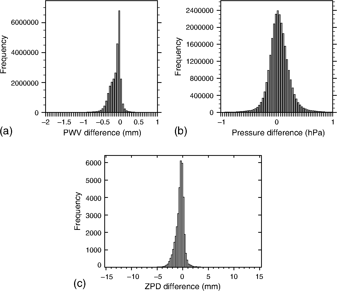
1.

Introduction

Synthetic aperture radar is a popular remote sensing technique for observing Earth’s surface. The strength of a signal, which is scattered back, is independent of the actual weather condition, whereas the wave propagation velocity depends on water vapor, pressure, and temperature.¹ Differential interferometric synthetic aperture radar (DInSAR) images are made from subtracted phase information from two synthetic aperture radar acquisitions and, therefore, are affected by weather changes. This spatial effect on the phases is known as the atmospheric phase screen (APS). Also affected is the absolute ranging technique, which considers the total delay of the waves instead of the phase.² In recent years, numerical weather predictions (NWPs) have become state-of-the-art in mitigating the atmospheric delays independent of the radar data. Different authors successfully demonstrated the mitigation of the APS using NWP for deformation estimation.^3–7 Similar to DInSAR, the delay correction using NWPs is also beneficial for the absolute ranging technique to estimate displacement maps.⁸ Cong et al.⁹ demonstrated a straightforward technique by using exclusively the European Centre for Medium-Range Weather Forecasts reanalysis (ECMWF ERA-interim) data, which are also used for the NWP initialization in this work. In comparison to this technique, the model-based prediction technique enables the physical interpolation between time steps. In case of ECMWF ERA-interim data, the time sampling is 6 h and a prediction interpolates temporally as well as spatially in a physically correct way.

Input weather data of a prediction are commonly of coarse resolution, and in this example it is 0.75 deg, which is $\approx 83\mathrm{km}$. Therefore, the initial data must be spatially interpolated for higher resolutions. This interpolation is physically unbalanced, as NWP needs prediction lead time to stabilize.¹⁰ This time is called spin-up time. The weather research and forecasting (WRF) model measures this imbalance by the diagnostic variable dpsdt, which is the domain averaged surface pressure tendency. This variable converges with further integration duration against a stable value, which represents the balanced state (see Fig. 2 at the end of this work). The imbalance disturbs the precipitation forecast at the first prediction hours.¹¹ This wrongly predicted precipitation disturbs the water vapor distribution, which causes zenith path delay (ZPD) prediction distortions, respectively. The digital filtering initialization (DFI) technique reduces this undesirable behavior^11–13 by integrating backward and/or forward in time, and removes nonphysical high frequencies by using a digital filter.¹⁰ This is particularly helpful for time-critical applications to save computational time. The DFI accuracy gain for ZPD predictions is unknown.

Similar to SAR acquisitions, Global Navigation Satellite System (GNSS)-measured time delays are also affected by the atmosphere and are very accurate and well investigated.^14–16 They provide the ground truth ZPD time series ($G_i$), because the best agreement between different approaches was achieved by the GNSS and the very long baseline interferometry (with a mean bias of $-3.4\mathrm{mm}$ and a standard deviation of 5.1 mm).¹⁵ For the accuracy gain investigation, the sample mean and the sample standard deviation of the residuals $D_i=F_i-G_i$ are computed, where $F_i$ is the predicted ZPD. The sample means and the sample standard deviations from residues ($D_i$) of WRF running with and without DFI are then compared.

The objective of this paper is to investigate the accuracy gain of delay predictions derived by the DFI technique, exemplarily at the test site in Germany.

2.

Methods

The ground truth in this work is provided by 233 GNSS stations mainly in Germany, their locations are displayed in Fig. 1(b). E-GVAP¹⁷ provides the corresponding ZPD time series ($G_i$) which were processed by GeoForschungsZentrum. Related to the GNSS time series, the WRF prediction data set consists of 44 predictions with and without DFI. The NWP dates are in-between 14 August, 2011, and 20 June, 2013. All 6-h predictions were initialized at 12 o’clock GMT, have a horizontal resolution of 2.7 km, and cover Germany. This is illustrated by the domain d02 in Fig. 1(a). ECMWF ERA-interim data¹⁸ with 0.75 deg resolution and 6-h time sampling were used as initialization data.

Fig. 1

(a) NWP domain configuration and (b) GNSS station locations.

The well-tested parameterization in Chapter 5 of the WRF User’s Guide was used.¹⁹ The actual three-dimensional state of the simulated atmosphere was sampled correspondingly to the ground truth $G_i$. A predicted ZPD time series $F_i$ with a time lag of 15 min was finally derived. This was achieved by the following integration, whereby the temperature as well as the water vapor data were trilinearly interpolated within the grid cells. For pressure, the horizontal data were bilinearly interpolated and, finally, exponentially interpolated in the vertical direction.

The predicted ZPD at time $i$ was computed by

The sample means and the sample standard deviations of the residuals $D_i=F_i-G_i$ are computed twice, one with and one without DFI. Respectively, both are compared for the accuracy gain investigation. That the DFI technique is useful for the ZPD prediction follows on from the fact that the DFI technique allows a more realistic initialization of cloud water content, precipitation, and vertical velocity fields.^11–13 The threat score, which is a measure for correctly predicted precipitation, is better if DFI is used.¹³ Since precipitation affects the water vapor distribution, it also affects the ZPD prediction and the related residuals. Correspondingly, the DFI technique reduces the residual $D_i$, which is shown in the following Sec. 3.1.

3.

Results

The accuracy gain investigation of the DFI ZPD prediction is divided into two parts. First, the accuracy gain is derived; second, the significance of the statistics is shown.

3.1.

Accuracy Gain Investigation

WRF predictions without DFI are affected more by physical imbalances in comparison to WRF predictions with DFI.^10,12,13 For the DFI predictions, 1-h backward integration, $1/2\text{-}\mathrm{h}$ forward integration, and a Dolph filter ($\mathrm{dfi}\_\text{nfilter}=7$) setting were used. The imbalance is measured by the diagnostic variable dpsdt and is averaged over the 44 WRF (version 3.5) predictions at different dates without DFI ($\mathrm{DFI}\_\mathrm{OPT}=0$) and with DFI ($\mathrm{DFI}\_\mathrm{OPT}=3$). Corresponding pressure tendency functions are shown in Fig. 2. The dashed line corresponds to WRF predictions with DFI and converges quickly against a stable value which represents the balanced state. In comparison, the solid line, which corresponds to the WRF predictions with common initialization, converges more slowly. Finally, both functions come close together at the fourth hour of the prediction. This point illustrates the average pressure tendency spin-up time of predictions without DFI.

The following accuracy gain investigation is divided into three parts. First, it is shown that the DFI results in a higher water vapor concentration than that of the common initialization. Second, it is shown that this DFI characteristic leads to higher ZPD predictions and, third, that this results in a lower ZPD bias.

Fig. 2

Domain-averaged surface pressure tendency.

3.1.1.

Digital filtering initialization effect on the water vapor concentration

It is known that WRF predicts too wet forecasts during the first 6 h of integration.²¹ It is also known that the threat score of precipitation forecasts is better if the DFI is used instead of the common initialization.¹³ In other words, the precipitation forecasts get better if the DFI is used instead of the common initialization. After the initialization, the model builds up clouds, i.e., water vapor condenses. The common initialization results in a higher cloud density and, correspondingly, in a lower water vapor concentration than the DFI. This is illustrated by the histogram in Fig. 3(a). Therefore, the precipitable water vapor (PWV) differences ${\widehat{R}}_i=R_i^{\mathrm{c}}-R_i^{\mathrm{d}}$ of the first prediction hour are computed, where $R_i^{\mathrm{c}}$ and $R_i^{\mathrm{d}}$ are the PWV data from the common and the DFI technique, respectively. This histogram shows that the PWV $R_i^{\mathrm{d}}$ is mostly slightly larger than $R_i^{\mathrm{c}}$ ($R_i^{\mathrm{c}}<R_i^{\mathrm{d}}$), because ${\widehat{R}}_i$ is mainly negative and close to zero. In other words, the DFI results mainly in higher water vapor concentrations than those of the common initialization.

Fig. 3

Difference histogram between the common initialization and the DFI predictions with respect to (a) PWV, (b) pressure, and (c) ZPD.

3.1.2.

Digital filtering initialization effect on the zenith path delay prediction

The ZPD $F_i$ can be divided into a hydrostatic $H_i$ and wet component $W_i$ by

Eq. (3)

$$F_i=H_i+W_i,$$

where $H_i$ is related to the first term and $W_i$ to the next two terms in Eq. (2). Thereby, $W_i$ is related to the PWV $R_i$ by the rule of thumb¹⁶

Eq. (4)

$$W_i=6.4R_i.$$

Since $R_i^{\mathrm{c}}<R_i^{\mathrm{d}}$ is mainly valid and because of Eq. (4), $W_i^{\mathrm{c}}<W_i^{\mathrm{d}}$ is mainly valid, where $W_i^{\mathrm{c}}$ and $W_i^{\mathrm{d}}$ are the wet ZPD components of the common and the DFI technique, respectively. Additionally, the hydrostatic component can be approximated by^22,23

Eq. (5)

$$H_i={10}^{-6}{K}_1\frac{R_{\mathrm{d}}}{g_{\mathrm{m}}}{P}_{\mathrm{s}},$$

where $R_{\mathrm{d}}=287.053\mathrm{J}{\mathrm{K}}^{-1}{\mathrm{kg}}^{-1}$, $g_{\mathrm{m}}=9.8\mathrm{m}/{\mathrm{s}}^2$ and $P_{\mathrm{s}}$ is the surface pressure in hPa. Similar to ${\widehat{R}}_i$, the surface pressure difference ${\widehat{P}}_{\mathrm{s}i}=P_{\mathrm{s}i}^{\mathrm{c}}-P_{\mathrm{s}i}^{\mathrm{d}}$ is computed, where $P_{\mathrm{s}i}^{\mathrm{c}}$ and $P_{\mathrm{s}i}^{\mathrm{d}}$ are related to the common initialization and the DFI, respectively. The corresponding histogram is shown in Fig. 3(b) and displays a centered Gaussian distribution with variance of $0.05{\mathrm{hPa}}^2$. Correspondingly, the hydrostatic ZPD change due to the DFI technique is negligible because of the tiny variance and Eq. (5). Consequently, the ZPD delay differences ${\widehat{F}}_i=F_i^{\mathrm{c}}-F_i^{\mathrm{d}}$, where $F_i^{\mathrm{c}}$ and $F_i^{\mathrm{d}}$ are related to the common initialization and the DFI, respectively, result mainly from PWV differences ${\widehat{R}}_i$. Therefore, the ${\widehat{F}}_i$ histogram in Fig. 3(c) has the same shape as the ${\widehat{R}}_i$ histogram in Fig. 3(a), and $F_i^{\mathrm{c}}<F_i^{\mathrm{d}}$ is mainly valid. In other words, the DFI ZPD predictions are inclined toward larger values than the common ZPD predictions.

3.1.3.

Digital filtering initialization effect on the biased zenith path delay prediction

Up to now, it has been shown that the DFI prevents a stronger condensation of water vapor than that of the common initialization, and results mainly in a higher ZPD prediction. The following shows that the structural higher DFI ZPD prediction reduces the bias of common ZPD prediction. Therefore, the residual $D_i$ sample means are shown in Fig. 4(a) depending on the forecast duration. The DFI sample mean is about 13% better than its counterpart during the first hour. This means that the bias is reduced if the DFI is used instead of the common initialization. This is also illustrated by the residual $D_i$ histogram in Fig. 4(b). The gray-colored histogram corresponds to the common initialization and the over-plotted histogram to the DFI technique. This shows that the gray histogram is more negatively biased than the over-plotted histogram.

Fig. 4

(a) The mean and standard deviation of the residual $D_i$ with respect to the integration hour and (b) the histogram of them for the first hour.

I do not compare the sample mean and standard deviation in time, because the accuracy is related to a time of day which influences the prediction accuracy. This is because heating or cooling effects are differently well presented relative to the time of day by WRF.

4.

Discussion

The ZPD bias reduction indicates a bias reduction with respect to the precipitation forecast. After the fourth hour of the prediction time, the accuracy gain of the DFI technique is vanished, which states that the precipitation forecast quality is then the same for both. Correspondingly, if the time of interest is from 4 to 6 or 10 to 12 either a.m. or p.m. GMT, then the DFI technique is not beneficial for the ZPD and precipitation prediction, because the ERA-interim time sampling is 6 h and starts at midnight GMT. In contrast to the means, the standard deviations in Fig. 4(a) of the DFI and the common initialization are close together. This means that the bias of the precipitation forecast is reduced but the uncertainty with respect to precipitation remains the same.

5.

Conclusion

The objective is to investigate the accuracy gain of predicted ZPDs by using the DFI technique at the test site in Germany. Finally, the following three implications are derived. First, the considered experiment confirms that the DFI technique improves the precipitation forecast because the negative bias of the residual $D_i$ is reduced. Second, the accuracy gain of the DFI is a 13% bias reduction of the ZPD prediction. Correspondingly, the biased position estimates, using the absolute ranging and the ZPD prediction technique, improve if the DFI technique is utilized. Third, if the SAR acquisition is from 4 to 6 or 10 to 12 either a.m. or p.m. GMT, then the needed prediction duration is larger than 4 h. Hence, the model is balanced anyway and thus the DFI accuracy gain is invalid. Correspondingly, the common initialization is recommended at that time to save computational time.