
|
|
1.IntroductionSatellite observations of the earth’s surface have been crucial for estimating biophysical and geophysical parameters used in a wide range of environmental studies.1 Estimation algorithms often involve algebraic manipulations of multispectral reflectance maps to provide scaler values that are strongly correlated with physical parameters.2–4 The spectral vegetation index (VI)4–6 is an example of an algebraic manipulation used routinely for a variety of purposes over several decades. These band manipulations have provided rich information from remotely sensed satellite imagery. Band manipulation is underscored by an assumption that if the parameter to be retrieved is fixed at a constant value, the reflectances measured at different wavelengths will be related.7,8 By limiting our discussion to the reflectance subspace formed by only two bands, the relationship of the reflectance spectra of the two bands form a line as a trajectory on the subspace. The relationship between two reflectances is defined as an “isoline” because a set of reflectance spectra on a true isoline corresponds to the same value of the retrieved parameter. Any successful retrieval algorithm should obtain indistinguishable retrieved results from all reflectance spectra on a true isoline. In general, knowledge of the relationship between two reflectances (isoline) plays an important role in an analysis of the performance of a retrieval algorithm.9–11 In the field of remote land sensing, vegetation isolines12 have been accepted as fundamental to VI equation models, especially given the uncertainties that can result from parameters unrelated to vegetation. Variations in the soil brightness beneath a canopy can significantly disrupt the VI, and such variations have attracted significant attention over time.12–20 These issues may be addressed using vegetation isolines to analyze the performances of VI estimation algorithms in the presence of soil effects. The concept of a vegetation isoline has often been invoked to minimize the influence of soil brightness. In recent years, the concept of an orthogonal vegetation isoline, the soil isoline,21–23 has been studied. The soil isoline is defined as a set of reflectance spectra attributed to a certain soil reflectance spectrum. The reflectance spectra on a given isoline result from a constant soil reflectance spectrum characterized by a unique set of soil optical properties. A soil isoline over the red and near-infrared (NIR) reflectance subspaces forms a single curve originating from a spectral point on a soil line.24–26 Soil line describes the linear relationship between the red and NIR reflectance spectra of a nonvegetated surface. Note that the soil isoline and the soil line are distinct concepts: the soil line is a special case of a vegetation isoline under “zero” vegetation conditions and it is obtained by varying the soil conditions. On the other hand, the soil isoline is obtained under constant soil conditions and variations in the biophysical parameters. Therefore, the soil line and vegetation isoline are similar concepts, whereas the soil isoline is orthogonal to the vegetation isoline and the soil line concepts. Because the vegetation isoline plays an important role in biophysical parameter retrievals, understanding the soil isoline contributes to a better understanding of soil optical property retrieval algorithms based on remotely sensed reflectance spectra. Equations describing the vegetation isoline have been extensively developed and used to analyze the VI,10 parameter retrievals,7 and the intercalibration of Vis.27–29 The soil isoline is not as popular a concept compared to the vegetation isoline, and it has not been studied analytically until recently. Numerical difficulties originating from a singularity associated with the polynomial fittings during the algorithms complicate the use of the soil isoline. In our previous work,30,31 a derivation technique was introduced to circumvent the singularity difficulties, and an analytical form of the soil isoline was derived and numerically validated. Previous studies derived the soil isoline under the assumption of full canopy coverage. In this case, the derived isoline equations are applicable only to regions in which a spatially homogeneous canopy covers the soil surface. These studies did not consider a heterogeneous target in which only a portion of the target region was covered by the canopy. Figure 1 shows a comparison of the soil isolines obtained from fully covered regions and partially covered regions in the red and NIR reflectance subspace. The figure clearly reveals the differences between the two cases (black line and gray line). These differences can introduce errors in subsequent analyses of the isolines if one does not distinguish the two cases. These cases may be treated appropriately by introducing a parameter that represents the fractional area covered by the canopy into the soil isoline formulations. This study attempts to do this using a parameter called the fraction of vegetation cover (FVC).4,9,32–35 Fig. 1Comparison of (solid black lines) the soil isolines for full canopy coverage conditions and (gray) soil isolines for partial (50%) canopy coverage conditions. The dotted line indicates the soil line in the red–NIR reflectance subspace. The green dot represents the convergent point for a fully covered dense canopy. Green circles , , and are those of partially covered canopies with different soil backgrounds, namely , , and , which denote the reflectance spectra of wet, moderately wet, and dry soil surfaces, respectively. Blue dots on the soil line are soil spectra without canopy. The gray dashed lines indicate the lines between the spectra for pure soil and fully covered canopy.  This paper describes the derivation of the soil isoline equations with consideration for the FVC. The objectives of this study are (1) to derive the soil isoline equations without truncating the polynomials; (2) to approximate the derived isoline equations for the sake of practicality by truncating the higher-order terms to obtain an analytical form of the red and NIR reflectance relationships under conditions of a constant soil reflectance spectrum; and (3) to validate the derived results by conducting a set of numerical experiments using a radiative transfer model to describe the coupling between the leaf and canopy layer system. The outline of the derivation appears first with a summary of the key findings of our previous work. Then we introduce model descriptions for an inhomogeneous system of vegetation canopy and soil surface, describe precise derivations and approximation cases, and provide numerical experiments by a radiative transfer model. Finally, we discuss the results by focusing on the accuracy of the derived and approximated soil isoline equations. 2.BackgroundThis section and Fig. 2 briefly summarize the four steps used to derive the soil isoline equation. The first step is transformation of an original red and NIR reflectance subspace into a new subspace. This transformation consists of rotation by the angle , defined as the slope of a soil line. The purpose of the transformation is to prevent singularities that might otherwise occur during the next step. The second step is determination of polynomial coefficients of the ’th-order term for each soil isoline in the transformed subspace. A relationship between red and NIR reflectance is represented along a soil isoline by a polynomial in the new subspace. The number of coefficient sets is identical to the number of soil isolines. The third step is the transformation of this relationship back into the original subspace to obtain a parametric representation of the soil isoline equation. The soil isolines are represented by power series of a common parameter. The final step is the approximation of soil isoline equations as relationships between the red and NIR reflectances of the original space by truncating the order of the common parameter. The approximated form of the soil isoline equation shows variation by the truncation order for each band. Hence, the accuracy of the derived isoline depends on the truncation orders of the two bands. Fig. 2Derivation steps of soil isoline equations in red and NIR reflectance subspace introduced in the previous study.31  3.Parametric Representation of the Soil Isoline Equations for a Partially Vegetated PixelThis section introduces the steps used to derive soil isoline equations that include a parameter to indicate the FVC, defined by . Please note that () represents the proportion of bare-soil within a target pixel. Therefore, the parameter “FVC” is tightly related to the soil parameter. In this context, it is quite natural to employ FVC in the soil isoline equations. Although the derivation described here is similar to the one introduced in our previous study for the case of full canopy coverage, care will be required to maintain consistency across the derived expressions and to clarify the differences between the fully covered and partially covered cases. 3.1.Linear Mixture Model of the Top-of-Canopy Reflectance Spectra of Partially Vegetated PixelsThe starting point of our derivation is the assumption of a linear mixture model (LMM) in which the top-of-canopy (TOC) spectrum is represented by a linear mixture of pure spectra known as endmember spectra.9 Although the assumption of a linear mixture is idealistic, it becomes a reasonably good estimate as the size of a target pixel gets larger. Thus, this assumption restricts the applicable range of this study to images acquired by satellites with moderate (15 to 30 m) to low spatial resolution. This study applied the two-endmember LMM in red and NIR reflectance subspace, denoted by the subscripts “r” and “n,” respectively. The subscripts “v” and “s” denote vegetation and soil, respectively. The TOC spectrum, , was defined as the weighted sum of the vegetated and nonvegetated spectra, defined by and , respectively. The TOC reflectance may then be expressed as We also assumed that the soil layer underneath the canopy was homogeneous over the entire target pixel. These assumptions enabled us to represent the well-known relationship between the red () and NIR () reflectances of the soil surface using a single soil line24–26 where and represent the offset and slope of the soil line, respectively. In this study, we explicitly differentiate the soil reflectance (, ) as an input parameter from the output reflectance spectrum (, ) of the soil line model.The next step involved applying an affine transformation to the TOC reflectance spectrum. This transformation was needed to avoid singular points in the numerical treatment of the soil isolines across a broader range of leaf area index (LAI). The details of this problem have been provided in previous studies.30,31 In this study, the affine transformation of a vector into is represented by the function , defined as where denotes the equal by definition. The angle , matrix , and vector are further defined by Note that the parameter represents the angle between the -axis and the soil line. Using these definitions, the transformed reflectance spectra of , , and could be written as Based on the linearity of the function , the following relation holds:The soil reflectance spectra became simple after the transformation because the transformed soil line was projected along the new red-axis where is the offset of the transformed soil isoline equation in the new subspace The TOC reflectance spectrum after the transformation could be written explicitly asEquation (13) suggested that the FVC parameter, , could be incorporated into the soil isoline equations describing the full canopy coverage with several modifications. Considering that the full canopy coverage is a special case of the partial canopy coverage, in which , the above analogy may be understood intuitively, and we may proceed with the derivation steps according to this analogy. 3.2.Soil Isoline Equations in the Transformed Subspacerepresents a single input parameter along the soil line. could be either , , or a ratio of wet and dry soil spectra. In either case, only a single parameter is needed to represent the model input. Therefore, we use in the rest of this study. The previous study proposed a polynomial fit as a function of the red soil reflectance as a representative of the soil brightness. By defining as a coefficient of the ’th-order term, was written as a polynomial of , such as The next step was to eliminate and from Eqs. (13) and (14). The result is an expression for the relationship between and , where represents the offset of the soil isolines, defined as Note that represents the offset of the soil isolines for the case of full canopy coverage in the transformed subspace. Because itself indicates the intersection between the transformed soil line and the transformed soil isolines, this offset is identical to Therefore, the offset of the soil isolines, , is simply the offset for the case of a full canopy coverage3.3.Parametric Representation of the Soil Isoline Equations for a Partially Covered CanopyIn the previous section, we derived the soil isoline equation in the transformed subspace. Next, we transformed the soil isoline equation back into the original red and NIR reflectance space. This process was performed by applying the inverse of the transformation Although Eq. (21) includes and as components of ; independently, can be written as from Eq. (16). Therefore, Eq. (21) can be written explicitly as a function of . Based on the relationship of Eqs. (16) and (19), the parametric form of the soil isoline equation [Eq. (21)] becameFor the sake of simplicity, we further introduced the following notation to describe the soil isoline equation where is a vector composed of the series , and and are vectors in a series of coefficients used to describe the polynomials of , defined as where the coefficients and are defined using the Kronecker delta Note that the zeroth-order terms of the polynomials describing each reflectance are equal to the spectra of the soil underneath the vegetation canopy Thus, all isolines approximated by any order will contain the true soil spectra and will agree exactly with the soil spectra, regardless of the approximation order, for the zero vegetation case.4.Approximations of the Soil Isoline EquationThis section introduces several approximate forms of the soil isoline equations, based on the introduction of various truncation terms in Eq. (24). Let us define the integers and as the polynomial orders employed in the red and NIR reflectances, respectively. The truncation terms could be explicitly differentiated by expressing Eq. (24) in the following form: where the function represents the contributions of the higher-order terms.The soil isoline equation could be approximated by choosing a pair of integers for and . Larger values would provide greater accuracy in the approximated soil isoline. The drawback, however, of choosing larger values for and is the increased difficulty associated with solving these equations for to derive analytical formulations of the soil isoline. In a previous study,31 we introduced a series of derivations to approximate the soil isolines by assuming full canopy coverage. In these derivations, the value of the FVC parameter did not appear explicitly in the study; nevertheless, it was considered as a special case in which the FVC was fixed to unity. Under these conditions, the following derivations are consistent with those described in our previous study. This point will be explored carefully below during the derivation steps. The analogy described above was used to guide the derivations first by simply enumerating the differences between the isolines of the fully covered case and of the partially covered case. We first clarified the differences between the coefficients defined in the previous study, and , and the coefficients defined in this study and . The major difference between the two cases (fully covered case and partially covered case) could be summarized in terms of the ratio of the coefficients and to their counter parts and , respectively, as follows: Because the differences only arose in the second- and higher-order terms, the approximated soil isoline equation could be modified under full canopy coverage conditions according to the following correction rules:4.1.Case-1 : First-Order Approximation of the Soil Isoline EquationThe first case to which the soil isoline approximation was applied comprised a model of the reflectance spectra in which only on the zeroth- and first-order terms were used to describe the red and NIR reflectances. This rule, summarized as (34) and (35), held that all coefficients (, , , and ) described in the previous studies remained unchanged. Therefore, the first-order approximated soil isoline equation was identical to the previously derived result Note that the approximated isoline did not include the parameter , indicating that this approximation was not suitable for conditions of partial canopy coverage. This parameter may be thought of as enhancing the nonlinearity of the soil isolines.4.2.Case-2 : Asymmetric First-Order-In-Red ApproximationIn this case, higher-order terms () were included in the NIR reflectance. Therefore, the influence of the FVC appeared in the NIR. The influence of these terms was explicitly differentiated by introducing a logical function in place of the integer , defined as This newly defined function was used to derive the soil isoline equation for a partial canopy coverage by applying the correction rule (34) and (35) to the results introduced in our previous work. We then obtained an approximated isoline where the coefficient is defined as4.3.Case-3 : Asymmetric First-Order-In-NIR ApproximationThis approximation case involved the same orders of approximation as case 2, except that the bands assigned to the first- and ’th-order approximations were reversed. The red reflectance was approximated by a higher-order polynomial (). The reciprocity resulting from the alternate band assignment yielded an equation for the approximated isoline where represents the coefficient of the ’th-order term describing the NIR reflectance, defined as4.4.Case-4 : Second-Order ApproximationThe second-order soil isoline included the FVC parameter in both bands because the second-order terms were influenced by the FVC. Application of the correction rule to the previously derived expression yielded the following result: where the function is defined as Note that only the last term depends on the parameter . Special caution is needed when one evaluates the above expression numerically because the denominator in contains , which can be equal to zero. As approaches zero, the reflectance spectrum on the isoline converges to the soil reflectance spectrum . Care is needed only in the context of numerical algorithmic treatments of this approximated form. This form of approximation is useful in a variety of applications, in addition to its utility in future studies.4.5.Case-5 : Higher-Order ApproximationThe last case comprises higher-order approximations in both the red and NIR bands. As described in a previous study, a rigorous solution to this approximation is impossible because the given equation cannot be solved for analytically. We circumvented this difficulty by including a higher-order term in the zeroth-order expression. In this way, we explicitly represented the higher-order contribution to the approximated formulation, as described in our previous study. As a result, the derivation was similar to the derivation introduced in Sec. 4.2, and the final approximation form became where is a coefficient (similar to ) that includes the index-like parasite parameter in the red reflectance, up to the ’th-order term and Note that the value of in Eq. (45) includes the parameter (in addition to the soil reflectance ), meaning that also depends on both and the biophysical parameter (LAI, in this study). This dependency distinguished this approximation case from the one introduced in Sec. 4.2.The expression for Eq. (45) could not immediately be used in numerical investigations because depended on itself, which could not be computed from Eq. (45). Nevertheless, the availability of this equation is beneficial to certain applications for which a good estimate of is available. One such application is the intercalibration of multiple sensors. For example, the spectral vegetation indices measured from two or more different sensors may be used simultaneously in a study, provided that the sensors are intercalibrated. In such applications, the value of for one sensor provides a good estimate of the other sensor’s corresponding band. The soil isoline equation of the higher-order case may be useful in practice for an intersensor calibration that involves hyperspectral sensors. In such an application, the availability of band reflectance (similar to a destination sensor) can be expected regardless of the band configuration of the multispectral sensor and hence relatively a lower order of terms would be required. As a result, without losing practicality, better accuracy would be expected from the use of a higher-order approximation of the soil isoline equation. 5.Numerical MethodThe validity of each derived soil isoline equation was evaluated using a series of numerical experiments involving a coupled leaf–canopy radiative transfer model, PROSAIL.36–38 To allow for a comparison between the current evaluation results and our previous study results (obtained from the fully covered case), the experimental conditions were set equal to those used in the previous study (Table 1). Table 1Input parameters of PROSAIL assumed in this study.
Special caution is needed in treatment of the FVC value in this study. The meaning of is an aerial proportion of a target region that can be represented by the PROSAIL model. When the LAI is less than unity, the true FVC value becomes less than unity within the homogeneous canopy region simulated by PROSAIL. Therefore, the actual FVC value over the entire region becomes smaller than when the LAI value is less than unity. By use of this definition, we maintain consistency with the derivation and numerical results of the derived soil isolines in the case of a fully covered canopy. Three PROSAIL parameters were varied during the experiments: the LAI, soil mixture ratio between the wet and dry soil spectra included in PROSAIL, which basically determined the soil brightness, and the FVC. PROSAIL was used to simulate the TOC spectra of the vegetated portion of the target area, and these spectra were then linearly mixed with the soil reflectance spectra to model the TOC spectra of the partial canopy coverage. We assumed a spherically uniform value for LAD, and the 10 and 30 deg angles were set as the view-zenith and illumination angles, respectively. The nominal parameter sets used to describe the leaf chemical content reported in Ref. 31 were applied in the current experiments. These simulation steps are summarized in Fig. 3. The reflectance spectra collected from the vegetated area could be obtained as an output from PROSAIL. The wavelengths of the output reflectance fell in the range 400 to 2500 nm. This spectrum depended only on LAI, the soil brightness, and FVC in this study. Next, the reflectances of the red and NIR bands were simulated at 660 and 850 nm, respectively, based on the band center wavelength of GOSAT-CAI (Greenhouse Gases Observing Satellite-Cloud and Aerosol Imager). The pure reflectance from a bare soil surface (a representative nonvegetated surface) was also simulated based on a linear sum of two standard soil spectra included in PROSAIL. An LAI of 0 to 4 at 0.8 intervals was set. Note that the approximated coefficients depended somewhat on the maximum value of LAI. In practical applications involving actual satellite images, these coefficients should be optimized using a training data set with known biophysical parameters and soil properties. A relationship between LAI and FVC was not assumed during the simulation. Thus, both LAI and FVC were mutually independent in this study. The FVC (varied from 0.0 to 1.0) was defined as the ratio of an output from PROSAIL to the bare soil spectrum. The spectra obtained from the two-band LMM depended on the soil brightness, LAI, and FVC. These simulated TOC reflectance spectra were considered to be the true spectra in this study. Most of the variables used in the approximated isolines were set equal to the corresponding values introduced in our previous study (of a fully covered case). Therefore, the steps of preparing the variables used in the isoline equations were almost the same as those applied in the case of full canopy coverage. In the case of full canopy coverage, the variables used in the soil isoline could be determined by following four steps: (1) retrieving the soil line parameters (slope and offset) from the reflectance spectra of the bare soil surface, (2) applying an affine transformation to the numerically simulated reflectance spectra, (3) fitting the transformed spectra along the soil isoline with a polynomial to obtain the fitting coefficients (), and (4) applying the inverse transformation back to the original red–NIR reflectance subspace to obtain the coefficients of the soil isoline equations (, ). The variables in the soil isoline equation for the case of partial canopy coverage were then computed by combining the parameter with the variables prepared according to the above four steps. The validity of the expressions derived in the previous section was tested by evaluating nine approximate cases defined by different pairs of and , representing the order of the terms used for the red and NIR bands, respectively. We assumed values of 1 to 3 for both and , which resulted in nine combinations. Table 2 lists the expressions used to approximate the soil isolines in this study. Table 2Summary of the approximated soil isoline equations used in the numerical experiments.
6.Results and DiscussionFigure 4 shows plots of the soil isolines simulated numerically by PROSAIL and those approximated using the expressions derived for fully covered and partially covered canopy cases. The marks denote the true reflectance spectra along each soil isoline, whereas the lines represent the soil isolines approximated by the derived expressions. The isolines were obtained by assuming three different soil brightness values for two approximation cases defined by two pairs of and . The figure indicated that the approximated soil isolines were close to the true isolines, even for the case of partial canopy coverage. At the same time, the choice of and influenced the accuracy of the isolines (the difference between the marks and lines). These results qualitatively suggested the validity of the derived expression. We next conducted a quantitative evaluation of the soil isolines. Fig. 4Comparisons between the approximated soil isoline equations and the “true” reflectance spectra simulated by PROSAIL. (a) The isolines approximated based on the truncation orders and , and (b) the isolines approximated based on the truncation orders and . The solid lines denote the case of (fully covered case), and the dashed lines denote the case of (partially covered case). The isolines for three types of soils with different brightness values (wet, intermediate, and dry) are shown in each case. 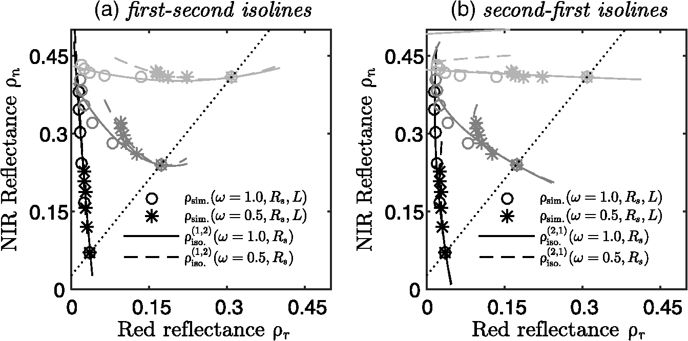 The accuracy of each of the nine soil isoline approximation cases was defined as the difference between the simulated spectra (considered to be the true spectra in this study) and the approximated isolines. Figure 4 shows the isolines and simulated spectra obtained for an FVC value of 0.5 or 1.0 at three soil brightness levels for (left) and and (right) and . As shown in Fig. 4, the accuracy of the isoline depended on the choice of the integer pair for and . This trend should be clarified quantitatively. The error was defined as the norm of the vector spanned by the simulated spectra and the derived isolines characterized by and . As a result, may be expressed as a function of FVC , the soil brightness , and LAI may be denoted , as Figure 5 shows plots of the distance profiles of the approximated isolines and the true spectra. The distances were plotted as a function of LAI and soil brightness (soil reflectance of the red band), and the value of FVC was assumed to be 0.5 for all plots. The order of the error was clarified by presenting the plots on the logarithmic scale. The nine plots were arranged from top to bottom (row-wise) for different choices of . The plots were arranged from left to right (columnwise) for the values of as well. The figure shows that the distance became shorter (hence, the error became smaller) as the choice of both and increased. These results indicated that the approximate soil isolines were better for the cases involving higher-order truncations, indicating the validity of our derivation. Fig. 5Error associated with the approximated soil isolines for nine combinations of the truncation order. The error is plotted as a function of LAI and soil brightness (soil reflectance of the red band). The FVC parameter was fixed to 0.5 during the simulations.  Figure 6 shows plots of the average differences between each isoline as a function of the FVC and soil brightness for the nine cases. The figures clearly indicated that the errors remained mostly stable, meaning that the order of the error generally depended on the order of the truncation. Moreover, the approximated isoline derived in this study nicely followed the variations in FVC. Fig. 6Plots of the mean absolute differences (MAD) between each soil isoline as a function of the FVC and soil brightness, for nine combinations of the truncation order. 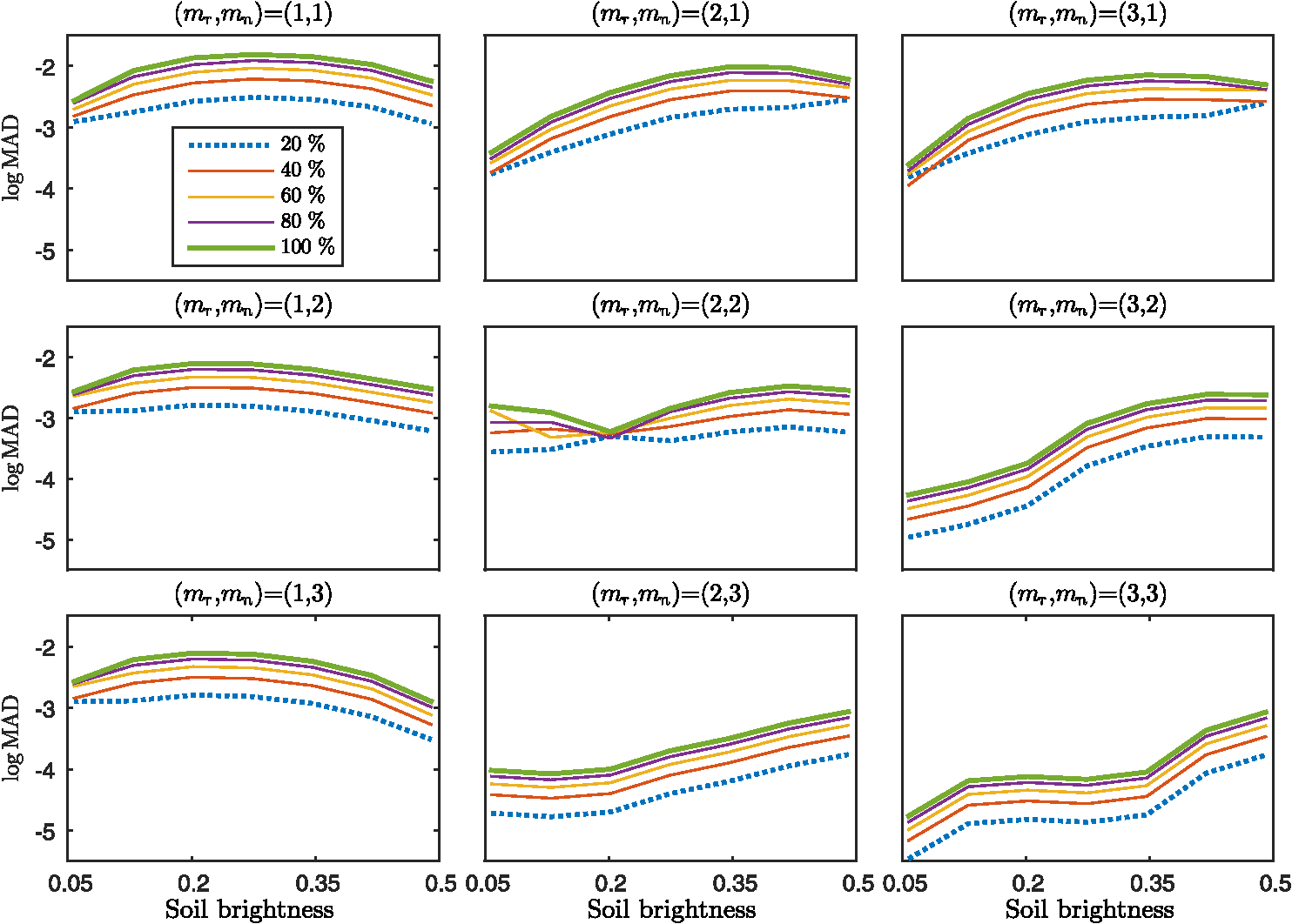 The overall trend in the error was confirmed by plotting the trends in the error and the standard deviation (STD). Figure 7 shows the averaged error and the STD for each isoline for all cases. The overall trend in the relationship indicated that the STD decreased as the error decreased. Considering the effects of the FVC, the error of the smaller FVC resulted in a smaller STD. These results implied that the maximum error and STD tended to occur at the highest FVC value. Fig. 7Overall score of MAD (bar) and an STD (line) for each soil isoline equation derived with the combination of polynomial orders . The bars and lines in green are the score for 100% canopy coverage, while those in blue are for 50% canopy coverage.  The overall averaged error and STD values for each case are summarized in Table 3. Three different LAD values (spherical, planophile, and erectophile) were compared to elucidate the influence of these values on the error and STD. The results revealed that both the error and its STD were reduced along with the higher-order terms in the approximated soil isolines. These results confirmed the validity of the derived expressions. Table 3Mean error of the approximated soil isoline equations for the three cases of LAD; (a) spherical, (b) planophile, and (c) erectophile.
The results of this study, based on comparison of the results of our previous study which assumed a fully covered canopy, indicate that the accuracy of the soil isoline equation improves when the vegetation coverage becomes smaller than unity. This is because the contribution of the canopy layer becomes smaller as the FVC value becomes larger; we implicitly assumed that the soil line used in this study includes no error. In reality, a soil line always includes a certain degree of uncertainty when the slope and offset are determined numerically. This implies a limitation of the derived soil isoline equations. The derivation assumes a certain model for the soil reflectance spectrum, so errors in the soil model would propagate into the soil isoline equations. This effect of soil model uncertainties should be investigated thoroughly in a future study. At the same time, accommodation of a better soil spectral model should also be explored. 7.Concluding RemarksThis study extends the previously derived soil isoline equations in the red–NIR subspace derived for the case of full canopy coverage. The parameter FVC was considered by employing the two-endmember LMM. Because the model used the FVC parameter explicitly in its formulation, we were able to derive the parametric form of the soil isoline equations using the FVC. The derivations proceeded by carefully noting the differences between the fully covered case and the partially covered case in the definitions of the isoline coefficients. We found that the FVC parameter contributed to the coefficients of the second- and higher-order terms for both the red and NIR bands, indicating that the FVC parameter only influenced the higher-order terms. These findings influenced the derivation of the four approximated cases defined over a range of truncation orders in the red and NIR reflectances. The validity of the derived expression was investigated by conducting a series of numerical experiments using PROSAIL. The numerical results revealed that the errors in the approximated isolines were reduced as the truncation order increased. These results clearly indicated that the isoline equations could be improved by accounting for the FVC parameter explicitly. Further validation efforts are needed to demonstrate the utility of this isoline model in analyzing satellite imagery. Such efforts will be considered in future work. AcknowledgmentsThis work was supported by the JSPS KAKENHI Grant Numbers 15J12297 (KT) and 15H02856 (HY). ReferencesC. J. Tucker, J. R. Townshend and T. E. Goff,
“African land-cover classification using satellite data,”
Science, 227
(4685), 369
–375
(1985). http://dx.doi.org/10.1126/science.227.4685.369 SCIEAS 0036-8075 Google Scholar
J. Clevers,
“The derivation of a simplified reflectance model for the estimation of leaf area index,”
Remote Sens. Environ., 25
(1), 53
–69
(1988). http://dx.doi.org/10.1016/0034-4257(88)90041-7 Google Scholar
E. P. Crist and R. C. Cicone,
“A physically-based transformation of Thematic Mapper data—the TM Tasseled Cap,”
IEEE Trans. Geosci. Remote Sens., GE-22
(3), 256
–263
(1984). http://dx.doi.org/10.1109/TGRS.1984.350619 Google Scholar
Z. Jiang et al.,
“Analysis of NDVI and scaled difference vegetation index retrievals of vegetation fraction,”
Remote Sens. Environ., 101
(3), 366
–378
(2006). http://dx.doi.org/10.1016/j.rse.2006.01.003 Google Scholar
A. Huete et al.,
“Overview of the radiometric and biophysical performance of the MODIS vegetation indices,”
Remote Sens. Environ., 83
(1), 195
–213
(2002). http://dx.doi.org/10.1016/S0034-4257(02)00096-2 Google Scholar
C. J. Tucker,
“Red and photographic infrared linear combinations for monitoring vegetation,”
Remote Sens. Environ., 8
(2), 127
–150
(1979). http://dx.doi.org/10.1016/0034-4257(79)90013-0 Google Scholar
A. Kallel et al.,
“Determination of vegetation cover fraction by inversion of a four-parameter model based on isoline parametrization,”
Remote Sens. Environ., 111
(4), 553
–566
(2007). http://dx.doi.org/10.1016/j.rse.2007.04.006 Google Scholar
M. M. Verstraete and B. Pinty,
“Designing optimal spectral indexes for remote sensing applications,”
IEEE Trans. Geosci. Remote Sens., 34
(5), 1254
–1265
(1996). http://dx.doi.org/10.1109/36.536541 IGRSD2 0196-2892 Google Scholar
K. Obata and H. Yoshioka,
“Comparison of the noise robustness of FVC retrieval algorithms based on linear mixture models,”
Remote Sens., 3
(7), 1344
–1364
(2011). http://dx.doi.org/10.3390/rs3071344 Google Scholar
H. Yoshioka et al.,
“Analysis of vegetation isolines in red-NIR reflectance space,”
Remote Sens. Environ., 74
(2), 313
–326
(2000). http://dx.doi.org/10.1016/S0034-4257(00)00130-9 Google Scholar
H. Yoshioka, A. R. Huete and T. Miura,
“Derivation of vegetation isoline equations in red-NIR reflectance space,”
IEEE Trans. Geosci. Remote Sens., 38
(2), 838
–848
(2000). http://dx.doi.org/10.1109/36.842012 IGRSD2 0196-2892 Google Scholar
A. R. Huete,
“A soil-adjusted vegetation index (SAVI),”
Remote Sens. Environ., 25
(3), 295
–309
(1988). http://dx.doi.org/10.1016/0034-4257(88)90106-X Google Scholar
A. J. Richardson and C. Weigand,
“Distinguishing vegetation from soil background information,”
Photogramm. Eng. Remote Sens., 43
(1977). Google Scholar
A. Huete,
“Soil-dependent spectral response in a developing plant canopy,”
Agron. J., 79
(1), 61
–68
(1987). http://dx.doi.org/10.2134/agronj1987.00021962007900010013x AGJOAT 0002-1962 Google Scholar
A. Huete, C. Justice and H. Liu,
“Development of vegetation and soil indices for MODIS-EOS,”
Remote Sens. Environ., 49
(3), 224
–234
(1994). http://dx.doi.org/10.1016/0034-4257(94)90018-3 Google Scholar
R. D. Jackson and A. R. Huete,
“Interpreting vegetation indices,”
J. Preventative Vet. Med., 11
(3), 185
–200
(1991). http://dx.doi.org/10.1016/S0167-5877(05)80004-2 Google Scholar
J. Qi et al.,
“A modified soil adjusted vegetation index,”
Remote Sens. Environ., 48
(2), 119
–126
(1994). http://dx.doi.org/10.1016/0034-4257(94)90134-1 Google Scholar
Z. Jiang et al.,
“Interpretation of the modified soil-adjusted vegetation index isolines in red-NIR reflectance space,”
J. Appl. Remote Sens., 1
(1), 013503
(2007). http://dx.doi.org/10.1117/1.2709702 Google Scholar
Z. Jiang et al.,
“Development of a two-band enhanced vegetation index without a blue band,”
Remote Sens. Environ., 112
(10), 3833
–3845
(2008). http://dx.doi.org/10.1016/j.rse.2008.06.006 Google Scholar
L. Montandon and E. Small,
“The impact of soil reflectance on the quantification of the green vegetation fraction from NDVI,”
Remote Sens. Environ., 112
(4), 1835
–1845
(2008). http://dx.doi.org/10.1016/j.rse.2007.09.007 Google Scholar
C. Atzberger and K. Richter,
“Spatially constrained inversion of radiative transfer models for improved LAI mapping from future Sentinel-2 imagery,”
Remote Sens. Environ., 120 208
–218
(2012). http://dx.doi.org/10.1016/j.rse.2011.10.035 Google Scholar
N. V. Shabanov et al.,
“Analysis and optimization of the MODIS leaf area index algorithm retrievals over broadleaf forests,”
IEEE Trans. Geosci. Remote Sens., 43
(8), 1855
–1865
(2005). http://dx.doi.org/10.1109/TGRS.2005.852477 IGRSD2 0196-2892 Google Scholar
N. V. Shabanov et al.,
“Analysis of interannual changes in northern vegetation activity observed in AVHRR data from 1981 to 1994,”
IEEE Trans. Geosci. Remote Sens., 40
(1), 115
–130
(2002). http://dx.doi.org/10.1109/36.981354 IGRSD2 0196-2892 Google Scholar
F. Baret, S. Jacquemoud and J. Hanocq,
“The soil line concept in remote sensing,”
Remote Sens. Rev., 7
(1), 65
–82
(1993). http://dx.doi.org/10.1080/02757259309532166 RSRVEP 0275-7257 Google Scholar
S. Jacquemoud, F. Baret and J. Hanocq,
“Modeling spectral and bidirectional soil reflectance,”
Remote Sens. Environ., 41
(2), 123
–132
(1992). http://dx.doi.org/10.1016/0034-4257(92)90072-R Google Scholar
J. C. Price,
“On the information content of soil reflectance spectra,”
Remote Sens. Environ., 33
(2), 113
–121
(1990). http://dx.doi.org/10.1016/0034-4257(90)90037-M Google Scholar
H. Yoshioka, T. Miura and A. R. Huete,
“An isoline-based translation technique of spectral vegetation index using EO-1 Hyperion data,”
IEEE Trans. Geosci. Remote Sens., 41
(6), 1363
–1372
(2003). http://dx.doi.org/10.1109/TGRS.2003.813212 IGRSD2 0196-2892 Google Scholar
H. Yoshioka, T. Miura and K. Obata,
“Derivation of relationships between spectral vegetation indices from multiple sensors based on vegetation isolines,”
Remote Sens., 4
(3), 583
–597
(2012). http://dx.doi.org/10.3390/rs4030583 Google Scholar
K. Obata et al.,
“Derivation of a MODIS-compatible enhanced vegetation index from visible infrared imaging radiometer suite spectral reflectances using vegetation isoline equations,”
J. Appl. Remote Sens., 7
(1), 073467
(2013). http://dx.doi.org/10.1117/1.JRS.7.073467 Google Scholar
H. Yoshioka and K. Obata,
“Soil isoline equation in red-NIR reflectance space for cross calibration of NDVI between sensors,”
in IEEE Int. Geoscience and Remote Sensing Symp. (IGARSS),
3082
–3085
(2011). http://dx.doi.org/10.1109/IGARSS.2011.6049869 Google Scholar
K. Taniguchi, K. Obata and H. Yoshioka,
“Derivation and approximation of soil isoline equations in the red–near-infrared reflectance subspace,”
J. Appl. Remote Sens., 8
(1), 083621
(2014). http://dx.doi.org/10.1117/1.JRS.8.083621 Google Scholar
M. F. Jasinski and P. S. Eagleson,
“The structure of red-infrared scattergrams of semivegetated landscapes,”
IEEE Trans. Geosci. Remote Sens., 27
(4), 441
–451
(1989). http://dx.doi.org/10.1109/36.29564 IGRSD2 0196-2892 Google Scholar
M. F. Jasinski and P. S. Eagleson,
“Estimation of subpixel vegetation cover using red-infrared scattergrams,”
IEEE Trans. Geosci. Remote Sens., 28
(2), 253
–267
(1990). http://dx.doi.org/10.1109/36.46705 IGRSD2 0196-2892 Google Scholar
T. N. Carlson, R. R. Gillies and T. J. Schmugge,
“An interpretation of methodologies for indirect measurement of soil water content,”
Agric. For. Meteorol., 77
(3), 191
–205
(1995). http://dx.doi.org/10.1016/0168-1923(95)02261-U 0168-1923 Google Scholar
T. N. Carlson and D. A. Ripley,
“On the relation between NDVI, fractional vegetation cover, and leaf area index,”
Remote Sens. Environ., 62
(3), 241
–252
(1997). http://dx.doi.org/10.1016/S0034-4257(97)00104-1 Google Scholar
W. Verhoef,
“Light scattering by leaf layers with application to canopy reflectance modeling: the SAIL model,”
Remote Sens. Environ., 16
(2), 125
–141
(1984). http://dx.doi.org/10.1016/0034-4257(84)90057-9 Google Scholar
S. Jacquemoud and F. Baret,
“PROSPECT: A model of leaf optical properties spectra,”
Remote Sens. Environ., 34
(2), 75
–91
(1990). http://dx.doi.org/10.1016/0034-4257(90)90100-Z Google Scholar
S. Jacquemoud et al.,
“PROSPECT+ SAIL models: A review of use for vegetation characterization,”
Remote Sens. Environ., 113 S56
–S66
(2009). http://dx.doi.org/10.1016/j.rse.2008.01.026 Google Scholar
BiographyKenta Taniguchi is a PhD student at Aichi Prefectural University, Aichi, Japan. He received his BS and MS degrees in information science and technology from Aichi Prefectural University in 2013 and 2015, respectively. Kenta Obata is a researcher at the Institute of Geology and Geoinformation at the National Institute of Advanced Industrial Science and Technology, Japan. He received his MS and PhD degrees in information science and technology from Aichi Prefectural University, Aichi, Japan, in 2010 and 2012, respectively. His research interests include intersensor calibration of biophysical retrievals, spectral mixture analysis, and radiometric calibration. Hiroki Yoshioka is a professor in the Department of Information Science and Technology at Aichi Prefectural University, Aichi, Japan. He received his MS and PhD degrees in nuclear engineering from the University of Arizona, Tucson, in 1993 and 1999, respectively. His research interests include cross-calibrations of satellite data products for continuity and compatibility of similar data sets and the development of canopy radiative transfer models and their inversion techniques. |
||||||||||||||||||||||||||||||||||||||||||||||||||||||||||||||||||||||||||||||||||||||||||||||||||||||||||||||||||||||||||||||||||||||||||||||||||||||||||||||||||||||||||||||||||


