|
|
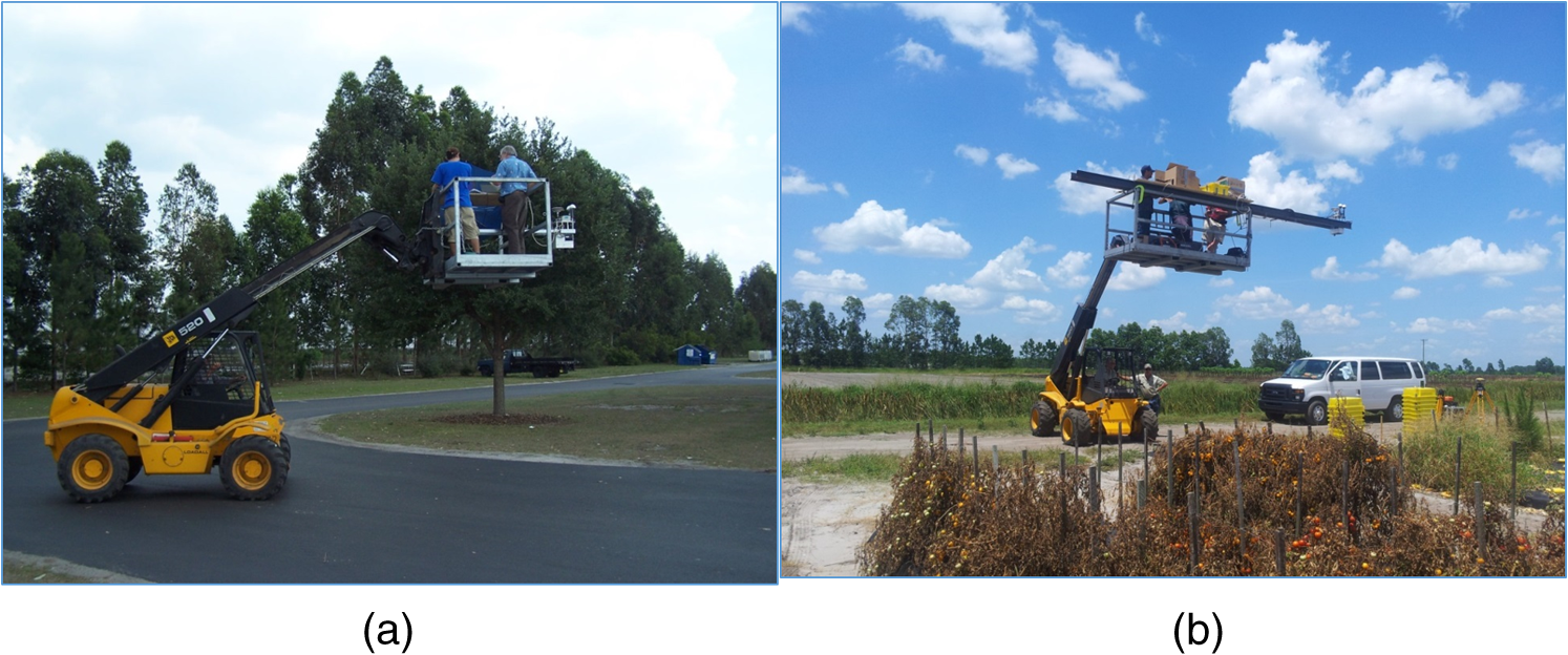
1.IntroductionRemote sensing imagery has been used extensively in agricultural applications such as plant stress detection, yield estimation, and field management. Foliage changes are often identified and modeled using spectral measurements.1–3 Stressed vegetation absorbs and reflects radiation differently along the electromagnetic spectrum causing symptoms that can be detected using spectral analysis.3–5 Specifically, changes in plant foliage due to different stress sources, such as diseases, nutrient deficiency, and drought, can be detected and quantified using spectral imaging. Using hyperspectral and multispectral imagery in agricultural field management is expected to continue to gain momentum as the sensors become more available and easier to deploy. Most hyperspectral imaging is performed using spaceborne and airborne platforms, which provide submeter and greater ground pixel size. Although the resolution range from these platforms is adequate for large area studies, it does not enable studies at the single-leaf or subcanopy level. Alternatively, close-range hyperspectral imagery taken from sensors mounted on agricultural farm equipment can efficiently provide finer spatial and spectral resolution imagery, as well as easy integration with daily agricultural operations.6,7 The introduction of small unmanned aerial systems (UASs) capable of carrying lightweight sensors should impact many of the agricultural applications of remote sensing. UAS imagery has finer spatial resolution compared to images captured by piloted aircraft. However, most UASs are relatively limited in payload capacity and are unable to carry substantial sensor packages. The increase in data quality, system reliability, and safety/operability aspects of ground-based systems normally provides great advantage and offsets any potentially higher cost due to the use of high-end equipment in such systems. Considering the regulations and reliability aspects of UAS, including the potential loss of expensive equipment, highlights the benefits of using ground-based systems. Accurate georeferencing of line-scanner hyperspectral imagery requires high-end inertial measurement units (IMU) and global navigation satellite system (GNSS) receivers in addition to synchronization mechanisms, which largely exceed the payload limitation of most small UAS. Ground-based systems can accommodate these needs as well as a whole suite of other sensors without the need to optimize for equipment size, weight, and power consumption, which can affect sensor performance and data quality considerably. There is a need for imagery with a resolution that is more than one order of magnitude higher than the resolution provided by UAS imagery. Close-range images captured per demand using ground platforms can provide the high spatial, spectral and temporal resolution that cannot be facilitated using traditional remote sensing techniques. In fact, the incomparably-high spatial resolution, the full control over temporal resolution, and the easy integration in agricultural operations of the mobile ground-based imagery enable a new set of applications, such as plant phenotyping, disease diagnosis, and per-demand real-time pesticide and nutrient application. Ground-based sensing technologies coupled with navigation sensors provide an optimal platform for high throughput data collection of the geometric, structural and spectral properties of plants.8,9 This type of data is necessary for utilizing precision agriculture technology at the large farm scale. Manual procedures to measure plants are well established; however, they are cumbersome, time consuming, and laborious.10 Using information collected with high spatial and spectral resolution ground-based imaging sensors provides an efficient solution to counter the limitations of traditional scouting and field sampling techniques. Image-derived measurements, such as canopy size and leaf reflectance, will not only improve agricultural capacity to monitor crop growth, model yield, and respond to plant stress and weed emergence in a timely manner, but further our understanding of the factors driving these processes for better management practices. Unlike traditional aerial images captured using stable nadir-looking platforms, ground-based images are subject to severe perturbations causing significant image distortion. Rigorous calibration must be included to evaluate and correct the geometric distortions in the imagery in order to facilitate image overlay and accurate stress quantification. This research provides a method for acquiring, georeferencing, and evaluating the accuracy of imagery collected using the mobile ground-based imaging system (MGIS). The MGIS is an integrated imaging system that includes a hyperspectral scanner7,11 with a GNSS receiver and an inertial navigation system (INS) in addition to a consumer grade single-lens reflex (SLR) digital camera. This system is designed to be a ground-based system for object and vegetation analysis (e.g., agricultural) applications.7 Hyperspectral image acquisition can be achieved using whiskbroom,12 pushbroom,13,14 and fixed focal plane15,16 sensors. Consumer-grade fixed focal plane cameras capture a two-dimensional (2-D) frame for each camera trigger and are often referred to as frame sensors. However, they suffer image distortion due to internal system instability and lens defects. The majority of contemporary hyperspectral sensors employ pushbroom image acquisition technology. For mobile pushbroom sensors, using direct georeferencing, direct observation of position and angular attitude of the sensor during acquisition is crucial to reconstruct the hyperspectral image cube line by line even with the existence of ground control points (GCPs). Thus, high-precision GNSS and INS observations must be acquired and integrated to provide accurate trajectory and hence image georeferencing. Successful implementation of ground-based imagery in plant phenotyping and stress detection applications requires accurate image georeferencing and geometric construction. The use of high-end navigation sensors (GNSS/INS) and appropriate synchronization mechanisms is important for any line-scanner sensor to achieve reliable images. For frame-based imagery, GNSS trajectories obtained through real-time kinematic or postprocessing techniques reduce the need for GCPs. Accurate trajectory also assists in the automated image matching process necessary for obtaining orthoimages and digital surface models (DSMs). Using ground-based high resolution imagery allows the collection of information at the individual leaf level. Such information enables detailed radiative transfer modeling and image radiometric calibration that cannot be performed without accurate geometric image construction. Although direct georeferencing of line scanners (including hyperspectral imaging systems) has been previously studied in the literature,17–19 most available research does not examine the georeferencing accuracy of ground-based hyperspectral imaging systems in an operational agricultural environment. Ground-based image acquisition involves driving the vehicle very slowly to ensure ground coverage on rough terrain to help mitigate the high level of platform vibration, which can potentially affect the observations of the GNSS/INS sensors. Such a harsh environment can affect the performance of individual system components as well, including imaging and sensors and synchronization equipment. In this context, the goal of this research is to introduce the mobile ground-based imaging system, a modular system composed of integrated off-the-shelf components in an agricultural field environment, and test the georeferencing accuracy of the acquired images. The MGIS system integrates a hyperspectral imaging sensor, a digital camera, and GNSS/INS navigation sensors to provide high-spatial resolution (1-mm pixel size) RGB orthoimages, and high spectral resolution (135 bands in the 400–900 nm spectrum) images. To the extent of the authors’ knowledge, no previous research has assessed the georeferencing accuracy of a ground-based imaging system such as the MGIS. To achieve the study goal, several images were captured over pavement and agricultural sites with established GCPs, and the positional accuracy of the resulting images was assessed. Section 2 of this manuscript describes system components, architecture, and the experiment study sites. Section 3 presents data preprocessing steps in preparation for the hyperspectral and digital camera image georeferencing process. Section 4 outlines the image georeferencing procedures including the theoretical background. Finally, Sec. 5 presents the georeferenced images and associated accuracy assessment. 2.System Configuration and Data Acquisition2.1.System ConfigurationThe MGIS is a modified version of the mobile mapping system introduced in Ref. 7. In the current version of the system, a NovAtel Span CPT GNSS/INS unit replaced the Gladiator LandMark 20 GPS/INS and Topcon Hiper Lite used in the previous system version. The hyperspectral sensor of the MGIS comprises a V10E Spectrograph integrated with an Imperx industrial camera. The spectrograph has a spectral range of 400 to 1000 nm and a 2.8-nm spectral resolution. The Imperx camera offers a resolution of . The hyperspectral sensor produces a final hyperspectral image cube with 800 spatial pixels (samples) and configurable (270 or 135) bands through 2, 4, or 8 pixel binning configuration.7 Also part of the MGIS is a Nikon D 300 DSLR camera synchronized to GPS time via GPS timing receivers. The hyperspectral and digital cameras were fitted inside a custom-designed aluminum housing. The GNSS/INS unit was installed on top of the housing, along with two GPS timing antennas that provide GPS time tags for the captured imagery, allowing synchronization with the trajectory information through GPS time. Figure 1 shows a schematic diagram of the system configuration. The whole system is composed of off-the-shelf components, as described in the study of Abd-Elrahman et al.7 The hyperspectral camera and the NovAtel Span CPT GNSS/INS comprise the most expensive components of the system. Each of these systems costs around $22,000. The remaining system components cost another $6000 to 10,000. It should be mentioned that some of these estimates are for academic use and do not include the cost associated with the image acquisition software and synchronization mechanism developed in-house. During the field data collection, the DSLR camera was set to take pictures at configurable acquisition rate through a custom-developed application, which could be used in future studies for digital elevation model (DEM) generation and/or updates to the trajectory. Two custom-made interface boxes were developed to trigger and time stamp the hyperspectral and DSLR camera imagery with GPS time using two Trimble Accutime Gold GPS receivers. Triggering signals are generated and controlled through custom applications developed using National Instruments Labview software for the hyperspectral sensor and the DSLR camera. Each GPS receiver is capable of timing events at an acquisition rate of 5 Hz or less. Considering the higher acquisition rate for the hyperspectral imagery (e.g., 40 Hz), the system is only capable of providing time stamps at a frequency that is less than the hyperspectral image acquisition rate. For example, if the hyperspectral image is acquired at 40 Hz (), only one in every eight acquired lines are tagged with GPS time. One of the subobjectives of this research is to test the georeferencing accuracy of the system characterized by this limitation. Each time a hyperspectral image frame is acquired, the data are transferred to the computer and the acquisition software reformats the individual frames to produce a hyperspectral image cube in a Binary Interlaced by Line (BIL) format. This image cube is then saved on the computer running the acquisition application. The DSLR camera imagery is stored on the camera flash drive to be retrieved after the imaging session. One of the main functionalities of the image acquisition software, in addition to sensor/camera trigger and saving the hyperspectral image, is to generate the time stamp log for the hyperspectral image and the DSLR camera frames. 2.2.Study SiteField measurements in the form of three MGIS scans took place at the University of Florida-Gulf Coast Research and Education Center (GCREC) in Wimauma, FL, and 82°13′40′′ W (Fig. 2). Two 100-m long stretches over pavement and agricultural beds were selected within the GCREC area. The MGIS was installed on a forklift tractor and set to capture data as it moved (Fig. 3). The first scan was collected over the paved road stretch [Fig. 2(a)] extending approximately in the east–west direction at 2:15 PM on June 4, 2014 (31°C and 43% humidity). Another two scans (scans A and B) were performed over a 100-m stretch of cucumbers and watermelon agricultural beds extending in the north–south direction [Fig. 2(b)] at 10:35 AM on July 1, 2014 (32°C and 45% humidity). DSLR images over the pavement lacked prominent features to support automated image matching necessary for processing, and thus were excluded from the analysis. It should be noted that choosing the scanned stretches to extend in east–west or north–south directions helped in debugging the results of the navigation data processing and image georeferencing steps, especially with the control point configuration extended along and off the scan trajectory line, as shown in Fig. 2. 2.3.Control Points and Lidar Data AcquisitionSeveral GCPs were established within each data collection site. Three GNSS receivers were set to collect static data for more than 4 h on control points labeled GCP_A, GCP_B, and GCP_C, established near the pavement road surface, as shown in Fig. 4(a). The same GNSS receivers were also set to collect static measurements exceeding 4 h on the control points labeled GCP_D, GCP_E, and GCP_F in the vicinity of the agricultural beds [Fig. 4(b)]. Sixteen control points were established on the pavement road surface, as shown in Fig. 5(a). The control point coordinates were surveyed using a total station by occupying GCP_C and backsighting GCP_A. Similarly, the total station was used to occupy GCP_D and backsight GCP_E to survey another 16 control points within the agricultural beds [Fig. 5(b)]. The GCP coordinates were in UTM zone 17 N (NAD83). Grid scale factor correction was applied to the total station measurements to account for the distortion associated with the map projection. Fig. 4Control points established using the GNSS receivers (a) near the pavement road surface and (b) within the agriculture beds. (Background images captured from Google Earth in 2014.)  Fig. 5Ground control points established using total station: (a) over the paved road surface and (b) within the agricultural beds.  A terrestrial laser scanner (lidar) was used to collect point cloud data for the paved road. The point cloud was used to create a DEM for image georeferencing. When performing the lidar scans, several spherical targets were placed on top of control points to allow georeferencing of the point clouds. The control points utilized in producing the processed lidar point cloud were measured independently from the total station GCP measurements, using GNSS receivers in static observation mode (1- to 3-h occupation time). 3.Data Processing3.1.Global Navigation Satellite System/Inertial Navigation System Trajectory PostprocessingThe MGIS hyperspectral sensor functions similar to most pushbroom sensors used in airborne and spaceborne remote sensing mapping applications, except this system is designed to capture ground-based images from an elevated mount on moving farm equipment. In order to process the GNSS/INS data correctly, three-dimensional (3-D) distance offsets (lever arm offsets) were measured to relate each sensor to the IMU origin. Offsets measured from the center of the IMU to the GNSS antenna were input to the GNSS/INS software in order to relate the GNSS antenna measurements to the IMU axis frame. Offsets were also measured from the center of the IMU to the hyperspectral sensor and DSLR camera. This allowed translation of the navigation data to the actual imaging sensor locations. Figure 6 shows the offsets from the IMU to the GNSS antenna and hyperspectral sensor. Two GNSS receivers were used to collect data at the GCP_A and GCP_B locations (independent of the observations used to generate the GCPs) while the MGIS scans were performed on the paved surface to enable differential correction. Similarly, two GNSS receivers were also set to collect measurements on the GCP_E and GCP_F control points located near the cucumber and watermelon agricultural beds site. The GNSS/INS data were processed using NovAtel Inertial Explorer. Output trajectories were produced at 100 Hz for each MGIS scan containing GPS time, latitude, longitude, pitch, roll, heading, and ellipsoidal heights. A custom script was developed to interpolate position and attitude angles for each captured DSLR camera and hyperspectral line image using the time stamp logs produced by the image acquisition software and the trajectory information exported from the Inertial Explorer software. 3.2.Digital Elevation ModelsConstructing a DEM is an essential step in georeferencing the collected hyperspectral images. The DEM used to process the hyperspectral imagery collected in the pavement stretch was constructed based on the lidar point cloud collected in the field. A simple DEM for the agricultural field was produced using control point elevations observed at the beginning and end of the beds. This configuration seemed reasonable given that bed preparation is conducted using machinery that employs GPS technology for leveling. In the future, we envision obtaining an accurate DEM as an output of the field preparation step conducted at the beginning of the crop cycle, mostly using GNSS-assisted machinery, such as tractors. 4.Image Georeferencing4.1.Hyperspectral Image GeoreferencingThe Parge20 orthorectification add-on to EXELIS ENVI 4.8 was utilized to georeference the hyperspectral images. The georeferencing process starts with importing the raw image cube and defining the DEM. Trajectory information is input as an ASCII file containing position (latitude, longitude, and height) and attitude angles (pitch, roll, and heading) of each line in the hyperspectral cube. GCP coordinates are used to compute the boresight angle offsets, defining the angular attitude of the sensor relative to the IMU coordinate system. Alternatively, georeferencing can be performed using predetermined boresight offsets without the need for GCPs. The equations describing scanning geometry have been derived by Ref. 21 and further refined by Ref. 22. As described in Ref. 20, the geometric model applied in Parge starts with the scan vector , as shown in Fig. 7. The same figure shows the initial coordinate system, which corresponds directly to image coordinate system, having the ; (sample) direction across track and the ; (line) direction along track. The initial scan vector for each pixel can be derived from the pixel scan angle assuming the across track vectors lie in a coplanar system. This is shown in the three equations listed below:20 where is the relative scan angle between pixel scan vector and nadir, is the sign (negative for left-hand side in the traveling direction pixels), and and are the across track and along track tilt of the sensor relative to the horizontal components of the navigation coordinate system (boresight offset angles in the roll and pitch directions), respectively. The sensor coordinate system is then rotated parallel to the ground space coordinate system. This rotation leads to new coordinates of the scan vector : where and are the rotation matrices for the attitude angles roll , pitch , and true heading , respectively. The , and matrices are defined asTo get the real length of the scanning vector , the scan vector length has to be related to the altitude of the MHIS as follows: Parge uses a statistical approach based on GCPs to calculate individual offsets for roll and pitch. For every GCP, the difference between known and estimated GCP position is calculated using the collinearity condition. By rotating the coordinate system back to the heading direction, the offsets for roll angle and pitch angle can be calculated for every GCP.20 Within the software main processor algorithm, the image geometry is calculated and the nearest neighbor interpolation option is applied to resample the output georeferenced hyperspectral image to the DEM grid.23 4.2.DSLR Image ProcessingAgisoft PhotoScan was used to process the DSLR camera data. Following the collection and organization of camera data, processing consists of four essential components: (1) initial image matching and orientation (alignment), (2) triangulation via bundle adjustment, (3) DSM generation, and (4) orthorectification. The initial image matching phase determines the location of conjugate points between multiple stereo images, from which the relative positions and angular orientation of all photos can be estimated. GCP coordinates and/or GNSS/INS observations associated with the camera are then used to establish the absolute position and angular orientation of the camera exposure stations via bundle adjustment. In order to obtain the best accuracy, camera calibration can also be included as unknowns in the triangulation/bundle adjustment phase and resolved in the solution. Once the absolute image geometry and camera calibration parameters are established from triangulation, fine-scale point clouds can be created using this information and a second denser image matching process. From the dense point cloud data, a DSM can be formed. Finally, orthophoto mosaics, dependent on both the absolute image geometry and DSM from previous steps, are produced via backprojection from the DSM to the images, a process called orthorectification. Orthorectified, mosaics consist of combined images corrected for the effects of camera tilt and distortions caused by topographical relief. In contrast with “rubber-sheeting,” using simple 2-D transformations to approximate map geometry, orthophoto mosaics are formed using statistically rigorous photogrammetric methods. They can be considered spatially accurate maps and reliably used to obtain planimetric measurements. A total of 85 DSLR camera images were processed to produce an orthorectified mosaic of the cucumber beds. As indicated earlier, the DSLR camera was mounted with the hyperspectral and navigating sensors on the forklift tractor at about 4 m above the agricultural bed. The coordinates of each camera exposure position were included in the photogrammetric solution. Two solutions and orthorectified mosaics were produced. One solution was generated using all 16 GCPs, and the other using only two control points at each end of the beds (a total of four control points). Using control points at the start and end of the beds, where minimal farming operations occur, is feasible in typical farming operations. The accuracy of these solutions based on checkpoints is presented in Sec. 5. 5.Results and Analysis5.1.Boresight Calibration of the Hyperspectral ImagesFailing to account for the pitch and roll boresight offsets in the hyperspectral image, georeferencing process has a great effect on the image positional accuracy. Table 1 presents the horizontal positional accuracy evaluated using the georeferenced hyperspectral images captured at the pavement site before and after performing the boresight angle calibration. The table shows the difference between the GNSS/total-station surveyed control point coordinates and the ones extracted from the georeferenced images. Root mean square error (RMSE) values of 0.083 and 0.142 m were calculated for the easting and northing coordinates, respectively, without boresight calibration. In this case, individual coordinate differences in the easting (approximately along track direction) are consistently negative with small standard deviation. Given the flat surface nature of the study site, this may be attributable to systematic error in image synchronization or pitch angle boresight offset. However, the effect of image synchronization offset may not be significant though due to the low speed of the moving platform (about 0.3 to ). Table 1Horizontal positional accuracy assessment of the pavement hyperspectral image before and after applying the boresight calibration.
The errors in the northing (across track) direction before applying the boresight calibration are also consistently negative. However, they vary among the three groups of control points located approximately north and south of the trajectory line. For each of these groups, the error values are similar in the easting direction, while the magnitudes of the northing errors differ from one group to the other. This observation highlights the boresight error in the across track direction and potential errors in the platform or DEM. Similarly, Tables 2 and 3 show the horizontal positional accuracy for the hyperspectral images captured in the first and second scans of the agricultural field with and without boresight calibration. The RMSE shown in Table 2 of the without-boresight calibration results is 0.123 and 0.115 m in the easting and northing coordinates, while Table 3 shows RMSE values of 0.101 and 0.097 m for the same component directions. The results shown in Tables 2 and 3 for the positional accuracy without applying the boresight calibration indicate consistently positive values for the calculated coordinate differences in the easting direction while the coordinate differences calculated in the northing direction are shown to be consistently negative. This pattern matches the one observed for the pavement scan, considering the prominently east–west direction of the pavement scan line compared with the north–south scan direction of the agricultural fields and highlights the existence of significant boresight angle offsets. Table 2Horizontal positional accuracy assessment of the first hyperspectral image in the agricultural bed before and after applying the boresight calibration.
Table 3Horizontal positional accuracy assessment of the second hyperspectral image in the agricultural bed before and after applying the boresight calibration.
The Parge software was used to calculate the boresight offsets using image and trajectory data in addition to ground control coordinates. These offsets have to be estimated and set once per flight or at least once per mission.23 The platform carrying the MGIS had nominally linear trajectories, following the same general direction from the beginning until the end of each scanning session. The effect of the heading boresight angles within each scan was determined to be very small. Accordingly, the effect of heading offset was considered negligible in this study. In fact, when accounting for the heading angle offset, the calculated accuracy was almost identical to that obtained when using only the roll and pitch boresight offsets. The roll and pitch offsets computed at each of the 16 control points in the pavement stretch are shown in Table 4. The table displays average roll and pitch offset values of 2.0 and , respectively. These values were calculated by averaging the roll and pitch offset determined for each control point listed in the table. Table 4Roll and pitch boresight offsets calculated for the pavement surface using all 16 control points, along trajectory centerline control points, and two control points only.
Comparing the roll boresight offsets estimated for the point groups north and south of the trajectory line, we noted that the roll offset values of each group were similar, having standard deviations that did not exceed 0.2 deg. Similarly, roll and pitch boresight offsets were calculated using only the control points located along the trajectory centerline and using only two control points (ECP and MCP) located at the eastern and western sides of the pavement scan to explore the potential of using fewer control points instead of the laborious 16 points used earlier. Table 4 shows roll offset angles of 1.8 and 2.0 deg and pitch offset values of and for the two cases. The roll and pitch values shown in the table indicates a 0.2-deg difference, which can result in 0.014-m error in the easting and northing directions at 4-m sensor elevation above ground. For the two MGIS hyperspectral images collected in the agriculture field, two of the control points established at the beginning and ending of the agriculture beds were utilized in the offset calculations for each scan. Table 5 displays the roll and pitch offset values of 1.7 and 1.2 deg, respectively, calculated for the data collected in the first agriculture field scan. These values were obtained by averaging the roll and pitch offsets at control points 2-M-3 and 15-M-3, as shown in Table 5. The table also shows roll and pitch offset values of 1.5 and , respectively, calculated for the second MGIS scan in the agriculture field, which were obtained by averaging the roll and pitch offsets calculated using control points 6-M-1 and 15-M-3. It should be noted that control point 6-M-1 was used instead of 2-M-3 in the roll and pitch offset calculations for the second scan line since control points 1-E-3, 2-M-3 and 3-W-3 were not visible in the hyperspectral images of the second scan line of the agriculture field due to inadvertent termination of the image acquisition process at the end of the scan line. Table 5Boresight offsets calculated using two control points for the two images collected in the agriculture field.
5.2.Horizontal Positional Accuracy Assessment of the Georeferenced Hyperspectral Images after Including the Boresight OffsetsThe horizontal positional accuracy of the georeferenced hyperspectral images acquired on the pavement stretch after applying the boresight calibration is shown in Table 1. These results were achieved by including the roll and pitch boresight calibration offsets estimated using control points MCP and ECP, as discussed in the previous section. The MCP and ECP control point coordinates were excluded from the accuracy calculations, as shown in Table 1. The table shows RMSE value of 0.015 m calculated for the easting coordinates and 0.031 m RMSE for the northing direction. The higher errors in the northing (across track) direction may be attributed to systematic errors in the sensor height above ground. This can lead to magnified error levels in the north–south (across track) direction compared to the errors in the east–west (along track) direction due to the existence of control points to the north and south of the trajectory line and the possibility that this error was absorbed in the pitch boresight offset determination process. This is evidenced by the consistently negative and positive values of the errors in the northing coordinates of the points located to the north and to the south of the trajectory, respectively. Table 2 shows the horizontal positional accuracy evaluated within the hyperspectral images captured in the first scan of the agricultural beds when performing the boresight calibration. RMSE values of 0.024 and 0.027 m are shown for the easting and northing coordinates, respectively. Similarly, Table 3 shows the horizontal positional accuracy evaluated for the hyperspectral images captured in the second scan of the agricultural field when implementing the boresight calibration. Calculated RMSE values of 0.023 and 0.025 m are shown for the easting and northing coordinates, respectively, which are comparable to those obtained for the first agricultural beds scan. The similarities between the error values calculated for the agricultural field scans are expected since the same DEM was utilized to process both datasets. However, these two scans were acquired using two independent trajectories and image data collection sessions. Such consistency increases the confidence in the obtained results given the harsh environment, exemplified by the tractor vibration and the rough ride, encountered during the agricultural field data collection sessions. Figure 8 shows two subsets of the georeferenced hyperspectral image for the road and first agricultural bed image. The images were produced (resampled) at 1-cm spatial resolution and some of the control points and land features (e.g., manhole on the asphalt in the pavement image) are visible. 5.3.Horizontal Positional Accuracy Assessment of the Georeferenced Digital SLR ImagesThe results of the bundle adjustment of the DSLR camera images are presented in Table 6. The table shows the results of the solution using all 16 control points and using only two points at each end of the beds. A RMSE value of 0.004 m was obtained in both easting and northing directions in the former case. The RMSE values for the four-control-points case (0.016 and 0.026 m in the easting and northing directions, respectively) were significantly more than the case when all 16 control points were used. However, as stated before, using several control points along an agricultural bed is not practical, especially when human labor and machinery are active. The proposed points can be established at the beginning of the crop season and used throughout the season for all imaging sessions. Table 6Horizontal accuracy assessment of the orthorectified image created from the DSLR images.
Our experimentation to solve the bundle adjustment using only direct georeferencing (no GCPs) resulted in a poorly resolved camera distortion model. This problem can be somewhat mitigated if multiple overlapped imaging lines were used. Nevertheless, special consideration should be taken in the image planning process as the shadow of the platform can consistently show in the images and causes the automated image matching to fail. 6.DiscussionOur results demonstrate successful implementation of a high spectral and spatial resolution ground-based mobile mapping system for agricultural applications. In this study, we used the higher-end SPAN CPT GPS/INS system instead of the lower-end Gladiator IMU7 to achieve reliable hyperspectral imagery in a rugged environment, such as the agricultural landscape. The use of the SPAN CPT system was seamless and did not affect the image acquisition workflow. Although there were previous attempts to develop and implement similar systems,7,9,24 most previous research only listed the specifications of the used components and did not test the georeferencing accuracy of the developed systems. Our research not only demonstrated the possibility to get superior spectral and spatial resolution imagery to assist agricultural operation and examined the positional accuracy of the system output but also documented the analysis workflow using commercial and in-house software. These study results showed that only a few control points are sufficient to achieve around 2.5 cm RMSE in the easting and northing directions for the hyperspectral and DSLR-derived orthoimages. The low number and distribution of the used control points demonstrate the operational use of the system in a typical crop agricultural field, where human and machine traffic can hamper the establishment of an extensive and season-long control point network. We recommend conducting a similar experiment using the specific conditions and equipment configuration used in the field to calibrate the system before each major acquisition. It is also advised to have redundant control points set aside for independent accuracy assessment of each mission. As mentioned earlier, the authors are not aware of other research evaluating the positing accuracy of ground-based systems and hence, we do not have similar reference to which we can compare our results. However, our results may be compared to airborne systems with similar sensor configuration considering the differences in flying height. For example, the RMSE achieved for the ground-based hyperspectral images are comparable to the 2.31 and 2.06 m RMSE in the easting and northing direction obtained using the self-calibrated direct georeferencing approach applied to airborne hyperspectral imagery with ground sampling distance of 1.2 m, as presented in Ref. 25. Similarly, an RMSE of about 2.4 m was reported for the airborne hyperspectral images analyzed in Ref. 26, which have 1.2-m pixel size. In this study, we analyzed the georeferencing accuracy of the hyperspectral and DSLR imagery independently using common navigation data. We believe that our results can likely improve with less reliance on control points if the information in both types of images were integrated, since the high-spatial resolution images can provide valuable surface model to assist the hyperspectral image georeferencing. Other future research may focus on reducing the need for inertial data through georeferencing the hyperspectral image directly to the DSLR-derived orthoimages, which can eliminate the need for inertial data. We believe that the promise of this system relies on future research at the application side (e.g., plant phenotyping, disease detection, yield modeling, etc.) that capitalizes on the achieved georeferencing accuracy and the ability to capture images recurrently. 7.ConclusionsGround-based hyperspectral and DSLR images were acquired using a system composed of integrated off-the-shelf components. The positional accuracy of the resulting imagery was assessed on a smooth paved road and rough agricultural field. The data collected from the field experiments were postprocessed to create georeferenced hyperspectral images with high spectral and spatial resolution. The integrated system was shown to be reliable by enabling the collection and analysis of several navigation datasets and multiple image sets synchronized using custom-made hardware and software components. The control points established in each study site were used to evaluate the positional accuracy of the MGIS data and to estimate the boresight calibration angles. The coordinates of the GCPs extracted from the georeferenced images were compared to the control coordinates measured independently using ground surveying techniques. The maximum RMSE obtained for the hyperspectral images in all experiments were 0.024 and 0.031 m in the easting and northing directions, respectively, when correcting for the boresight offsets. These results were achieved using only two control points at both ends of the scan line to estimate the boresight calibration offsets. The RMSE values of the orthorectified mosaic constructed using DSLR camera images and two control points at each end of the agricultural site were 0.016 and 0.026 m in the easting and northing directions. Operationally, establishing control points at the start and end of the agricultural beds is considered convenient to avoid along bed potential disturbance due to farm equipment. ReferencesJ. Torres-Sánchez et al.,
“Configuration and specifications of an unmanned aerial vehicle (UAV) for early site specific weed management,”
PLoS One, 8
(3), e58210
(2013). http://dx.doi.org/10.1371/journal.pone.0058210 POLNCL 1932-6203 Google Scholar
J. M. Peña et al.,
“Weed mapping in early-season maize fields using object-based analysis of unmanned aerial vehicle (UAV) images,”
PLoS One, 8
(10), e77151
(2013). http://dx.doi.org/10.1371/journal.pone.0077151 POLNCL 1932-6203 Google Scholar
H. Li et al.,
“Extended spectral angle mapping (ESAM) for citrus greening disease detection using airborne hyperspectral imaging,”
Precision Agric., 15
(2), 162
–183
(2014). http://dx.doi.org/10.1007/s11119-013-9325-6 Google Scholar
C. Bing et al.,
“Spectrum characteristics of cotton canopy infected with verticillium wilt and applications,”
Agric. Sci. China, 7
(5), 561
–569
(2008). http://dx.doi.org/10.1016/S1671-2927(08)60053-X Google Scholar
R. A. Naidu et al.,
“The potential of spectral reflectance technique for the detection of grapevine leafroll-associated virus-3 in two red-berried wine grape cultivars,”
Comput. Electron. Agric., 66
(1), 38
–45
(2009). http://dx.doi.org/10.1016/j.compag.2008.11.007 CEAGE6 0168-1699 Google Scholar
X. Ye et al.,
“A ground-based hyperspectral imaging system for characterizing vegetation spectral features,”
Comput. Electron. Agric., 63
(1), 13
–21
(2008). http://dx.doi.org/10.1016/j.compag.2008.01.011 CEAGE6 0168-1699 Google Scholar
A. Abd-Elrahman, R. Pande-Chhetri and G. Vallad,
“Design and development of a multi-purpose low-cost hyperspectral imaging system,”
Remote Sens., 3
(3), 570
–586
(2011). http://dx.doi.org/10.3390/rs3030570 RSEND3 Google Scholar
H. Wang et al.,
“Image-based 3-D corn reconstruction for retrieval of geometrical structural parameters,”
Int. J. Remote Sens., 30
(20), 5505
–5513
(2009). http://dx.doi.org/10.1080/01431160903130952 IJSEDK 0143-1161 Google Scholar
D. Deery et al.,
“Proximal remote sensing buggies and potential applications for field-based phenotyping,”
Agronomy, 4
(3), 349
–379
(2014). http://dx.doi.org/10.3390/agronomy4030349 AGRYAV 0065-4663 Google Scholar
R. T. Furbank and M. Tester,
“Phenomics-technologies to relieve the phenotyping bottleneck,”
Trends Plant Sci., 16
(12), 635
–644
(2011). http://dx.doi.org/10.1016/j.tplants.2011.09.005 Google Scholar
R. Pande-Chhetri and A. Abd-Elrahman,
“Filtering high-resolution hyperspectral imagery in a maximum noise fraction transform domain using wavelet-based de-striping,”
Int. J. Remote Sens., 34
(6), 2216
–2235
(2013). http://dx.doi.org/10.1080/01431161.2012.742592 IJSEDK 0143-1161 Google Scholar
G. Vane et al.,
“The airborne visible/infrared imaging spectrometer (AVIRIS),”
Remote Sens. Environ., 44
(2), 127
–143
(1993). http://dx.doi.org/10.1016/0034-4257(93)90012-M RSEEA7 0034-4257 Google Scholar
M. Wulder, S. Mah and D. Trudeau,
“Mission planning for operational data acquisition campaigns with the CASI,”
in Proc. of the Second Int. Airborne Remote Sensing Conf. and Exhibition,
24
–27
(1996). Google Scholar
J. S. Pearlman et al.,
“Hyperion, a space-based imaging spectrometer,”
IEEE Trans. Geosci. Remote Sens., 41
(6), 1160
–1173
(2003). http://dx.doi.org/10.1109/TGRS.2003.815018 Google Scholar
H. Saari et al.,
“Unmanned aerial vehicle (UAV) operated spectral camera system for forest and agriculture applications,”
Proc. SPIE, 8174 81740H
(2011). http://dx.doi.org/10.1117/12.897585 PSISDG 0277-786X Google Scholar
A. Makelainen et al.,
“2D hyperspectral frame imager camera data in photogrammetric mosaicking,”
Int. Arch. Photogramm. Remote Sens. Spatial Inf. Sci., XL-1/W2 263
–267
(2013). http://dx.doi.org/10.5194/isprsarchives-XL-1-W2-263-2013 1682-1750 Google Scholar
R. Muller et al.,
“A program for direct georeferencing of airborne and spaceborne line scanner images,”
Int. Arch. Photogramm. Remote Sens. Spatial Inf. Sci., 34
(1), 148
–153
(2002). Google Scholar
J. Perry et al.,
“Precision directly georeferenced unmanned aerial remote sensing system: performance evaluation,”
in Proc. of the 2008 National Technical Meeting of The Institute of Navigation,
680
–688
(2001). Google Scholar
C. K. Yeh and V. J. Tsai,
“Self-calibrated direct geo-referencing of airborne pushbroom hyperspectral images,”
in IEEE Int. Geoscience and Remote Sensing Symp.,
2881
–2883
(2011). http://dx.doi.org/10.1109/IGARSS.2011.6049816 Google Scholar
D. Schläpfer and R. Richter,
“Geo-atmospheric processing of airborne imaging spectrometry data. Part 1: parametric orthorectification,”
Int. J. Remote Sens., 23
(13), 2609
–2630
(2002). http://dx.doi.org/10.1080/01431160110115825 IJSEDK 0143-1161 Google Scholar
E. E. Derenyi and G. Konecny,
“Infrared scan geometry,”
Photogramm. Eng., 32
(5), 773
–779
(1966). PHENA3 0554-1085 Google Scholar
G. Konecny,
“Mathematical models and procedures for the geometric restitution of remote sensing imagery,”
in Invited paper of the XIII Int. Congress of Photogrammetry, Commission III,
33
(1976). Google Scholar
S. Sankaran, L. R. Khot and A. H. Carter,
“Field-based crop phenotyping: multispectral aerial imaging for evaluation of winter wheat emergence and spring stand,”
Comput. Electron. Agric., 118 372
–379
(2015). http://dx.doi.org/10.1016/j.compag.2015.09.001 CEAGE6 0168-1699 Google Scholar
C. K. Yeh and V. J. Tsai,
“Self-calibrated direct geo-referencing of airborne pushbroom hyperspectral images,”
in IEEE Int. on Geoscience and Remote Sensing Symp.,
2881
–2883
(2011). http://dx.doi.org/10.1109/IGARSS.2011.6049816 Google Scholar
R. Pande-Chhetri et al.,
“Classification of submerged aquatic vegetation in black river using hyperspectral image analysis,”
Geomatica, 68
(3), 169
–182
(2014). http://dx.doi.org/10.5623/cig2014-302 Google Scholar
BiographyAmr Abd-Elrahman is an associate professor at the University of Florida. He received his PhD in civil engineering with a concentration in geomatics from the University of Florida and his MS and BS degrees in civil engineering from Ain Shams University, Egypt. His research interest is in remote sensing and spatial analysis applications in natural resource management and precision agriculture. His research involves developing a mobile ground-based hyperspectral/multispectral imaging system for precision agriculture applications. Naoufal Sassi was employed at the New York State Department of Transportation for 4 years as transportation construction inspector (2007 to 2010) and then earned his Bachelor of Engineering degree in civil engineering from the University at Buffalo in 2011. He received his Master of Science degree with a geomatics concentration in 2014 from the University of Florida. While pursuing his degree, he worked as a research assistant for the University of Florida. Benjamin Wilkinson is an assistant professor at the University of Florida, specializing in photogrammetry and lidar. His focus is on developing methods for data adjustment and error propagation, and applying these to the fusion of multimodal data. He is a coauthor of the textbook Elements of Photogrammetry with Applications in GIS. Bon Dewitt received his PhD degree from the University of Wisconsin in 1989. His specialties include photogrammetry, surveying, and digital mapping. Currently, he is an associate professor and director of the geomatics program at the University of Florida and is a fellow member of the American Society for Photogrammetry and Remote Sensing. His primary research focuses on digital image sensor calibration and photogrammetric analysis of imagery from unmanned autonomous vehicles. |
|||||||||||||||||||||||||||||||||||||||||||||||||||||||||||||||||||||||||||||||||||||||||||||||||||||||||||||||||||||||||||||||||||||||||||||||||||||||||||||||||||||||||||||||||||||||||||||||||||||||||||||||||||||||||||||||||||||||||||||||||||||||||||||||||||||||||||||||||||||||||||||||||||||||||||||||||||||||||||||||||||||||||||||||||||||||||||||||||||||||||||||||||||||||||||||||||||||||||||||||||||||||||||||||||||||||||||||||||||||||||||||||||||||||||||||||||||||||||||||||||||||||||||||||||||||||||||||||||||||||||||||||||||||||||||||||||||||||||||||||||||||||||||||||||||||||||||||||||||||||||||||||||||||||||||||||||||||||||||||||||||||||||||||||||||||||||||||||||||||||||||||||||||