1.

Introduction

A major challenge for weather forecasting in mountainous areas is the need for high-density surface observations to resolve and to parameterize the fine-scale gradients of meteorological parameters produced by topographic and thermal forcing.¹ Assimilation of dense data also allows refinements of numerical weather prediction models for mountain weather applications.² The meso- and microscale weather models need better physical parameterizations of the atmospheric boundary layer (ABL) to resolve thermally and mechanically induced flows such as slope and valley flows, and boundary layer structures.^3,4 Under weak synoptic conditions, the diurnal wind circulations are topographically induced, and additional observational studies are needed to determine governing mechanisms of these ABL flows.⁵ In all, there is an urgent need for observational technologies that are accurate, high-density, nimble, and cover large spatial extents.

Observing ABL winds in mountainous areas, however, is challenging because of high spatial and temporal wind variability as well as the logistical difficulties of deploying in situ observing platforms. Rapid spatial variation of land cover, surface thermal gradients due to preferential solar heating, mechanical and thermal separated flows, and internal waves and intense turbulent regions all contribute to the measurement challenges of complex terrain.^6,7 Typically, tower-mounted sonic anemometers have been the measurement instruments of choice, but a large number of in situ probes are required for adequate spatial and temporal coverage. In many observational studies, this is not logistically and physically (tower interference) feasible, especially for observing upper levels of the boundary layer at the heights of several hundred meters, e.g., behind wind turbine blades. To this end, Doppler wind lidars (DWLs) offer a sound remote sensing technique for velocity measurements.

Most DWL use a coherent detection technique^8–10 in which the return signal of a pulsed laser beam scattered from aerosols is mixed with a reference laser beam of known frequency. The effect of multiple scattering is minimized in the design due to the small field of view of the laser beam. An onboard signal processing computer determines the Doppler shift from the spectra of the signal, and calculates the radial velocity of air along the beam as averaged over certain distance windows or range gates. As such, the coverage of DWL measurements depends on aerosol loading in the atmosphere. Two lidars (dual) intersecting at a given location provide two velocity components within the probe volume, whereas three (triple) lidars yield all three velocity components.

The classical single radar velocity azimuth display (VAD)¹¹ and volume velocity processing (VVP)¹² techniques assume a horizontally uniform flow within the scanning cone (for VAD) or a uniform flow in a sector of the scanning volume (for VVP), and the wind speeds and directions are derived by fitting a sinusoidal curve through the radial wind data; many variants of single lidar retrieval algorithms are based on this assumption. Single DWLs have been extensively used in ABL studies for both flat and gently variable terrain,^13–19 over urban areas,^20–23 and for studies on wind turbine wakes at heights of hundreds of meters.²⁴ While the assumptions used for single DWL retrievals are appropriate for many situations, they are not suitable for highly complex and spatially variable turbulent flows in mountainous terrain. The advent of dual lidar wind retrieval was a significant step forward in measuring the real wind fields, and has been used for measurement of mean horizontal wind fields and turbulent structures^25,20 and for virtual towers of mean horizontal winds²¹ by assuming that the mean wind is parallel to a nearly flat ground surface with negligible vertical motions. Dual DWLs have also been used to retrieve horizontal winds and vertical profiles of horizontal winds²⁶ using a variational retrieval algorithm. In a strict sense, however, this technique is only suitable for nearly two-dimensional flows. To observe the true wind vector more accurately, three lidars are needed, the implementation of which is the topic of this paper.

The coordinated scanning of three DWLs can cover a continuum of lidar intersection points (probe volumes) over a relatively large atmospheric volume with relatively high spatial resolution. This allows the retrieval of all three components of wind velocity without invoking assumptions on the flow at the probe volume. This triple lidar technique was attempted during the mountain terrain atmospheric modeling and observations (MATERHORN^27,28) program, wherein ABL measurements were made in complex terrain using a suite of remote sensing assets and in situ probes. This paper reports on the efficacy and utility of coordinated triple lidar deployments for three-dimensional (3-D) turbulent wind observations in the ABL. The turbulence information derived from triple DWL is evaluated and tested against the data from colocated standard sonic anemometers, and comments are made on the feasibility of the triple DWL technique as a future standard ABL measurement platform.

Measurement of ABL turbulence using DWL has been a challenging problem. Most of the previous studies have assumed a specific turbulence model for retrievals. For example, the turbulent kinetic energy (TKE) dissipation rate and structure function have been recovered from raw radial velocity data using the assumption of isotropy in the Kolmogorov inertial subrange^29,30 or using large-eddy simulation techniques.³¹ Collier et al.²⁵ described a variety of quantities derivable from lidar measurements, such as rms velocities, TKE dissipation rate, and convection velocities, again by invoking turbulence models. Choukulkar et al.³² used DWL measurements to derive dispersion parameters based on eddy diffusivity assumptions. Nevertheless, a universally agreeable model of turbulence covering all scales does not exist. A detailed review on turbulence measurement using DWL is given in Sathe and Mann.³³

The coordination of synchronized triple DWLs in a static staring mode has been recently reported for ABL wind and turbulence measurements in nearly flat terrain.^34,35 In this work, Mann et al.³⁴ analyzed the DWL signal attenuation in its resolvable wave numbers due to spatial averaging within the range gates. Fuertes et al.³⁵ developed a spatial filtering technique that allows comparison of sonic and triple DWL-derived turbulence spectra and fluxes for large turbulent eddies without using a turbulence model. These two studies have demonstrated that synchronized triple DWL staring at a spatial point has the potential to observe large turbulent eddies, but the present study demonstrates an even greater potential of triple DWL; to derive 3-D wind vectors at various locations over a large spatial volume when all three lidars are continuously scanning in a coordinated manner.

In this paper, we employ synchronized triple lidar data taken during the MATERHORN experiment, during which a number of lidar configurations were evaluated. The triple Doppler lidar-derived turbulence signal is evaluated and tested against colocated data from standard sonic anemometers. The feasibility of measuring the mean 3-D wind vector using triple lidars in a coordinated scanning mode is also evaluated by comparison with a nearby sonic anemometer.

2.

Wind Vector Retrieval from Triple Doppler Wind Lidar

The mathematics of retrieving a 3-D wind vector from triple lidar radial velocities is quite straightforward, and involves a transformation from an arbitrary laser-beam coordinate to a Cartesian coordinate. Here, we use the directional cosine approach, in preference to the alternative Euler angle or polar coordinate to Cartesian transformation approaches.³⁶ If one considers a wind vector at a point in two reference coordinate frames, the vector can be represented in either reference frame and there is a unique transformation between the two reference frames. The triple lidar 3-D wind vector is represented by three independent radial velocities, $V_j=(V_1,V_2,V_3)$, and it can be transformed from a Cartesian coordinate $U_i=(U_1,U_2,U_3)$ with east ($x$), north ($y$), and up ($z$). This transformation can be expressed using the usual tensor

Fig. 1

A schematic diagram to indicate the laser beam in a local Cartesian coordinate (east, north, and vertical) and the directional angles (${\theta }_{11}$, ${\theta }_{12}$, ${\theta }_{13}$) for lidar 1. The point $(x,y,z)$ is where the three lidar beams meet (for clarity, the other two lidars are not shown).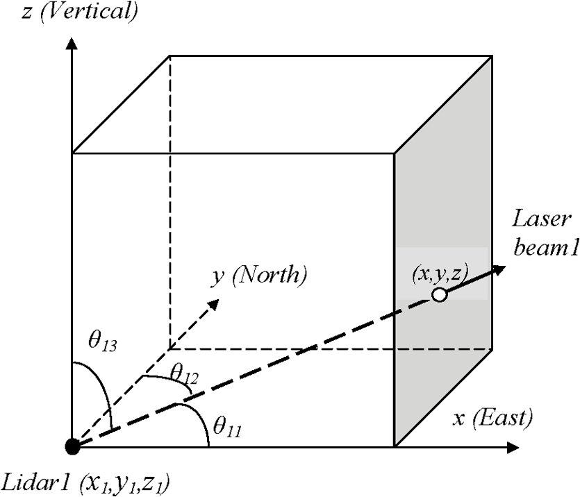

The local coordinates for all three lidar locations and beam meeting-points are computed via a geodetic transformation³⁷ using their latitudes, longitudes, and altitudes. Geodetic transformations map spatial points on the Earth to different coordinate representations. Specifically the local ENU (east, north, and up) system based on the lidar location is transformed into the GPS reading of latitude, longitude, and altitude for any spatial point or vice versa. It is emphasized here that the intersection point of the three lidar beams could be at any point in space, and a specific directional cosine matrix needs to be recomputed for each meeting point. One of the challenges of triple lidar wind-vector retrieval is the synchronization of all three beams to have a common meeting point in space at a given time. In our work, each of the three lidar scanners was independently controlled, making synchronization difficult. We first synchronized the three computer clocks for the data acquisition systems, and each radial velocity reading was stamped with a time, range gate, signal-to-noise ratio, and azimuth and elevation angle. When a 3-D wind vector was computed, all information from the lidar scanner and from the beam gate was used for synchronization and alignment purposes. For analysis of the staring data, the synchronization and alignment of laser beams was rather simple because the three stationary laser beams were pointed to a spatial point for a long period. Synchronization and alignment are more difficult when retrieving an instantaneous 3-D wind vector measured while the lidars are scanning, as in the case of a virtual tower. Obtaining three-beam intersections at a given spatial point at the exact same time is very challenging in this case. Thus, threshold values for time and spatial accuracy had to be set to ensure sufficient (approximate) synchronization and alignment. Such a threshold approach has been used previously for two-dimensional wind retrieval.²¹ For this study, we used threshold values of 5 s in time and 2 m in space. These threshold values are based on the limitations of the sampling frequency (0.25 Hz) and scanner resolution (0.5 deg) described in the next section.

3.

Instrumentation and Observational Sites

The measurements were a part of the MATERHORN field campaign, which is a comprehensive meteorological research program involving multiple university groups and national laboratories.^27,28 It was designed to identify and study the limitations of current state-of-the-science mesoscale models for mountainous terrain weather prediction, and to develop scientific tools to help realize major advancements in predictability. One of the core scientific objectives is to study fundamental near-surface exchange processes and to investigate the spatial and temporal variations of the ABL in complex terrain. A component of the project also concerned the development of new technologies and measurement methodologies for ABL probing, and our work falls into this category.

The observation site is located at the Granite Mountain Atmospheric Science Testbed (GMAST, centered at 40.125° N, 113.30° W) at the U.S. Army Dugway Proving Ground in Utah. The GMAST terrain ranges between $\sim 1300\mathrm{m}$ above sea level (ASL) over flat playas and 2159 m ASL over the rugged Granite Peak. There were two seasonal field campaigns, fall (October 2012) and spring (May 2013), each with ten 24- to 36-h-long intensive observation periods (IOPs). The fall campaign was focused on weak to moderate wind conditions, dominated by thermally driven (up/down slope and valley) flows while the spring campaign focused on the interaction of large-scale, synoptic weather systems with topography. A comprehensive data set was collected using an array of meteorological towers, ground-based DWLs, wind profilers, radiosondes, tethersondes, microwave radiometers, and an airborne DWL. A line of five towers (ES1 to ES5) running up the east slope of Granite Peak was especially relevant to our study of coordinated triple DWL observations. A detailed description of MATERHORN can be found in Fernando et al.²⁸

During both field campaigns, three scanning DWLs were used: a Leosphere WindCube100s operated by the U.S. Army Research Laboratory (ARL) and two Halo Photonics Stream Line lidars operated by the University of Notre Dame (UND) and the University of Utah (UU). The range resolution of the Halo lidars was 18 m, and the Leosphere lidars had a range resolution of 50 m. Signal-to-noise thresholds ($\text{Beta value}>{10}^{-7}$) for the Halo lidars and a carrier-to-noise ratio ($\mathrm{CNR}>-27\mathrm{dB}$) for the Leosphere lidar were also used for data screening. The detailed physical parameters of these two types of DWLs are listed in Table 1. During both the 2012 and 2013 field campaigns, the sampling frequencies were 20 Hz for sonic anemometers, 1 Hz for the ARL Leosphere lidar, and 0.25 Hz for the UU and UND Halo lidars.

Table 1

The system parameters configuration of the Leosphere Windcube 100S and the Halo Stream line DWL during MATERHORN.

The detection ranges were different for these two types of lidars, and for the GMAST site’s dry and clean atmospheric conditions, the range was $\sim 1\mathrm{km}$ for the Leosphere and $\sim 0.7\mathrm{km}$ for the Halos. A portion of the deployment time was devoted to developing and testing a methodology for using coordinated triple DWLs for turbulent wind observations over complex mountainous terrain, as described in this paper. The setup for May 15, 2013, is shown in Fig. 2 and for October 7, 2012, in Fig. 3. The geodetic coordinates were determined by GPS readings and the distances between the lidars were computed with a geodetic computation. The transformations between Cartesian and geodetic coordinates (latitude, longitude, and altitude) were performed using in-house developed software.³⁷ A special staring design was implemented on May 15, 2013, enabling comparisons between turbulence recorded by a sonic anemometer (R. M. Young 81000) and the lidars. The accuracy of the sonic anemometer is $0.05{\mathrm{ms}}^{-1}$ in wind speed and 2 deg in wind direction. In addition to the staring setup, a virtual tower configuration was employed during both the experiments (Figs. 2 and 3).

Fig. 2

May 15 to 16, 2013, setup of the three DWL from ARL (green), UND (blue), and UU (red). (a) A 3-D depiction of RHI scans of the three DWL. (b) A latitude, longitude, and altitude coordinate for the three DWL. Note that a meteorological tower (ES3) with a 20-m AGL sonic anemometer was located between the UND and UU lidars.

Fig. 3

October 7, 2012, setup of three DWL from ARL (green), UND (blue), and UU (red). (a) A 3-D depiction of RHI scans from the three DWL. (b) A latitude, longitude, and altitude coordinate for the three DWL. Note that a 32-m meteorological tower (ES2) with a 28-m AGL sonic anemometer was located between the UND and UU lidars.

The UND and UU lidar range height indicators (RHIs, a scan pattern with a fixed azimuth scanning between two designated elevations along a vertical plane) scanned in an approximately covertical plane, while the ARL lidar performed RHIs through this coplane at different locations. During May 15 to 16, 2013, the UND and UU lidars were programmed to scan 45 deg elevation RHIs in an east-west coplane while the ARL lidar scanned 45 deg RHI frames, intersecting with the UND/UU coplane at different locations. Such scanning permitted the retrieval of 3-D vectors from the radial velocities measured by three DWLs (Fig. 2). During the night of October 7, 2012, the three lidars were configured differently as shown in Fig. 3. The UND and UU lidar scanned 180 deg RHI in a nearly north-south coplane, while the ARL lidar scanned through this coplane at different locations to produce virtual towers. The scanning elevation angle interval for the Leosphere lidar was 1 deg and the Halo lidar was $\sim 0.8\mathrm{deg}$. The scanner angular speed was $1\mathrm{deg}{\mathrm{s}}^{-1}$ for the Leosphere lidar and $\sim 2.4\mathrm{deg}{\mathrm{s}}^{-1}$ for the Halo lidar. The lidar scanner elevation and azimuth angles were set by locating the geodetic coordinates of the lidar locations with a GPS, carefully leveling the lidars, and pointing the scanners to true north using a compass, taking into account the angle of declination. In order to reduce possible errors, the lidar orientation azimuth was checked with multiple compasses, and the terrain reference point at the starting beam line was checked with Google Earth software to verify the scanner azimuth orientation.

4.

Data and Analysis

4.1.

Observations of Large Turbulent Motions Using Dual Doppler Wind Lidar Via Staring

The triple DWL staring test was carried out during the night of May 15, 2013 (Fig. 2). All three lidars were pointed at the uppermost sonic anemometer (20 m AGL) of the ES3 tower, with the objective of comparing sonic and DWL measurements. Unfortunately, during the staring period, the data from the UND Halo lidar were lost due to a technical failure. Since the UND and UU Halo lidars are identical, we assumed that it would be adequate to compare only the UU lidar signal with the sonic anemometer.

Figure 4 is a time series plot of the horizontal and vertical wind speed and wind direction from the 20 m sonic anemometer at the ES3 tower on May 15, 2013. During the presented period, the winds are north-northwest with mean speed near $1.8{\mathrm{ms}}^{-1}$ between 0300 and 0430 UTC. After 0430 UTC, the wind direction is more variable and the wind speed increased to about $4.5{\mathrm{ms}}^{-1}$. This time series is in the ENU coordinate and is used to compare to the lidar wind observations by transforming the sonic anemometer wind components into the lidar radial wind directions. The time series is nonstationary. By applying Eq. (1), the ES3 sonic anemometer velocity components ($U_i$) were rotated to the reference frame of the lidar beams.

Fig. 4

Sonic anemometer observed time series of horizontal wind, vertical wind, and wind direction at 20-m AGL height on the ES3 tower on May 15, 2013. This time series is used to compare the lidar wind observations by transforming the wind components in the lidar radial wind directions.

Figure 5(a) compares the observed lidar radial wind component and the sonic anemometer wind component along the laser beams for the entire staring period. Further inspection shows that the DWL (red) and sonic anemometer (black) data track very closely. The sonic-based winds capture more fluctuations compared to the lidar data because of its ability to better resolve smaller turbulent eddies in the inertial subrange; the spatial resolution of the sonic anemometer ($\sim 10\mathrm{cm}$) is much higher than that of the lidars (range gate sizes: 18 m for the UU Halo and 50 m for the ARL Leosphere). Furthermore, a disparity exists in the temporal resolutions, although the Leosphere lidar (longer range gate of 50 m) is more capable of capturing higher frequency fluctuations than the Halo lidar due to a higher sampling frequency (1 versus 0.25 Hz). Neither lidar, however, can match the temporal resolution of the sonic anemometer (20 Hz). Table 2 lists the statistical values for these two pairs of time series. The mean, standard deviation, and the skewness compared well between the lidar radial velocities and the corresponding radial velocities from the sonic anemometers. All four time series showed positive skewness, reflecting upward spikes in the turbulent wind signal in Fig. 5. The comparison of sonic and lidar data is difficult because of the disparities of sensing volumes and data acquisition rates. We used the spatial filtering technique introduced by Fuertes et al.³⁵ to filter the sonic radial velocities, wherein no assumptions are made on the nature of turbulence. The spatial window of the filter is transformed from time to space domains by applying Taylor’s hypothesis. When analyzing a 12-min time segment [Fig. 5(b)], the effects of the lower resolution of the lidars are more visible. Since the range-gate size of the Leosphere lidar is more than twice that of the Halo and the signal was averaged with the larger range gate of the Leosphere, the radial wind of the latter followed the sonic anemometer more closely than the former. The spatially filtered time series of sonic radial velocity had a better agreement with those of the lidars (Fig. 5).

Fig. 5

Comparison between radial velocities ($V_{\mathrm{r}}$) for the ARL and UU lidars with the sonic anemometer at 20-m AGL on the ES3 tower on May 15, 2013. (a) A zoomed image between the green lines. (b) The cyan lines are spatial filtered radial velocities derived from the sonic anemometer using the technique of Fuertes et al.³⁵

Table 2

Comparison of statistical values between the sonic and lidar observed radial wind time series.

	Mean (ms−1)	Standard deviation (ms−1)	Skewness
ARL radial wind (lidar)	1.73	0.97	0.99
ARL radial wind (sonic)	1.90	1.00	1.26
UU radial wind (lidar)	$-0.28$	1.39	0.72
UU radial wind (sonic)	$-0.22$	1.21	0.80

It is instructive to compare the wind-component signals in the frequency domain since turbulent winds contain a vast range of scales and frequencies of turbulent eddies (in the presence of constant wind speed, by virtue of Taylor’s Hypothesis, the results can be construed in spatial or wave number terms). In this analysis, a time series of winds is transformed into a spectral representation using the Fourier transform^38,39

Eq. (3)

$$S(f)={\int }_0^{\infty }{R}_{\mathrm{a}}(t)\exp (-\text{if}t)\mathrm{d}t,$$

where $R_{\mathrm{a}}(t)$ is the auto-correlation function of the wind component $a$, $f$ is the cyclic frequency, $t$ is the time, and $S(f)$ represents the TKE per unit frequency at different frequencies. Figure 6 shows the spectra for the ARL (a) and UU (b) lidars and their comparisons with the colocated 20 m sonic anemometer at the ES3 tower. These spectra were computed using the entire time series of lidars, sonic anemometer, and spatially filtered sonic anemometer. The spectra from the filtered sonic radial velocities are slightly closer to the lidar radial velocity spectra (Fig. 6).

Fig. 6

Spectral domain comparison of DWL (black) and sonic anemometer (green) radial velocities taken at 0300 to 0500 UTC on May 15, 2013. The pseudospatially filtered sonic radial velocity spectra are shown in red. (a) Comparison of spectra between the sonic anemometer component and the Leosphere lidar. (b) Comparison of spectra between the sonic anemometer component and the Halo lidar. Arrows point to the Nyquist frequency ($f_{\mathrm{N}}$) of sampling, large energetic eddy frequency ($f_{\mathrm{e}}$), and resolvable frequency using Taylor’s hypothesis ($f_{\mathrm{r}}$) for the ARL and UU lidar data.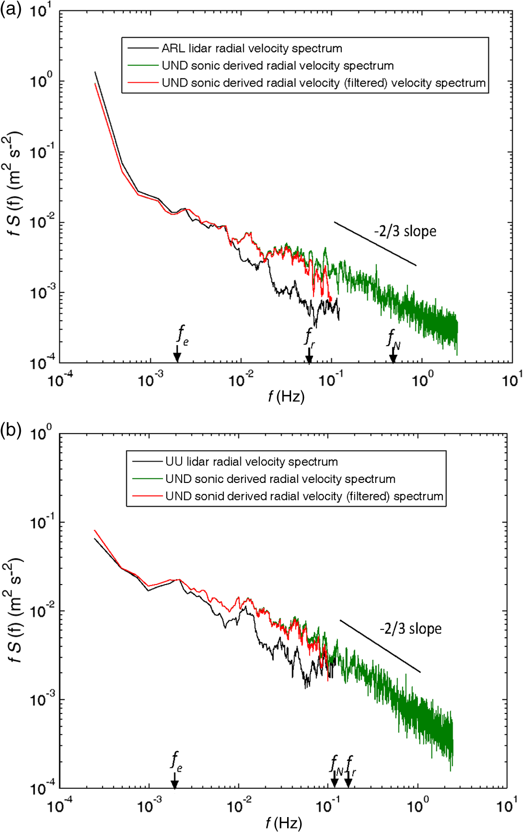

In interpreting Fig. 6, the following should be noted. First, the good agreement between the sonic anemometer and lidars in the low-frequency spectrum shows that large turbulent eddies are captured by the lidars well up to an energetic large-eddy frequency cut off ($f_{\mathrm{e}}=0.008\mathrm{Hz}$); a plot of $S(f)$ versus $f$ shows that most of the along-beam component energy ($\sim 79\%$ along the ARL lidar beam, $\sim 63\%$ along the UU lidar beam) is contained below the frequency of the “energy containing” eddies ($f<f_{\mathrm{e}}$) which is defined as the frequency corresponding to the maximum of the plot. Taking the typical mean velocity as $\overline{U}=3\mathrm{m}{\mathrm{s}}^{-1}$ (see Fig. 5), for this time series and using Taylor’s hypothesis, this translates into a relationship between the wave number ($k$) and frequency of $k\overline{U}=2\pi f_{\mathrm{e}}$ or an eddy size of ${\ell }_{\mathrm{e}}=\overline{U}/2\pi f_{\mathrm{e}}=60\mathrm{m}$, which is a reasonable value based on previous observations.³⁹ Second, note that the sampling Nyquist frequency ($f_{\mathrm{N}}$, defined as half the sampling frequency) for the UU lidar is 0.125 Hz and for the ARL lidar is 0.5 Hz, and frequencies higher than $f_{\mathrm{N}}$ are to be discarded for the lidar results. Third, the lidar radial velocity is spatially averaged by a weighting function which has a peak value at the center of a range gate; this spatial average is equivalent to spatial filtering with a filter function and the resulting radial velocity has fewer fluctuations than exhibited by the sonic anemometer. The spatial resolution of the lidar (range-gate size) imposes a restriction on the size of eddies that can be resolved. For UU, this is $k=2\pi /18=0.35{\mathrm{m}}^{-1}$, and hence above the frequency of $f_{\mathrm{r}}=k\overline{U}/2\pi =0.17\mathrm{Hz}$, which is slightly greater than its sampling Nyquist frequency. For the ARL lidar, the wave number $k$ becomes $2\pi /50=0.125{\mathrm{m}}^{-1}$ and $f_{\mathrm{r}}=0.06\mathrm{Hz}$. The limiting factor for the ARL lidar is its spatial resolution rather than the sampling frequency for this relatively low wind speed of $3{\mathrm{ms}}^{-1}$. We expect the classical Kolmogorov spectra [$-5/3$ slope, i.e., $-2/3$ slope for $f_{\mathrm{S}}(f)$] is applicable for $f_{\mathrm{r}}>f>f_{\mathrm{e}}$ sonic anemometer data, but the slope is slightly steeper for Doppler lidar data, reflecting the spectral attenuation due to the spatial average of the range gate (Fig. 6). A rough estimation can be made of the amount of energy that is becoming “opaque” because of the low resolution of the lidar. Integrating the spectrum up to $f=f_{\mathrm{r}}$, we find that TKE is underestimated in lidar measurements by about 7% for the ARL lidar, and 11% for the UU lidar compared with the sonic anemometer. Analogously, the work of Kit et al.⁴⁰ showed that about 10% of the energy is unaccounted for due to the relatively low resolution of sonic anemometers compared to hot-film probes.

4.2.

Mean 3-D Wind Retrieval Using Triple Lidars with the Lidars Scanning

The 3-D velocity vector retrieved from coordinated triple lidar measurements is an Eulerian observation, and our exploratory work was directed at observing vertical profiles of 3-D wind vectors at different heights while the lidars are scanning. As depicted in Figs. 2 and 3, the three lidars scanned in coordination to make three lidar beams cross the predetermined vertical lines at approximately the same time. These vertical profiles (or virtual towers) were realized by arranging the lidars in such a way that the UND and UU lidars scanned a coplane and the ARL lidar scanned through the coplane, cutting through the intersection. The synchronization proved to be very difficult, as the simultaneous intersection of all three laser beams (say, within $<1\mathrm{s}$) using individually controlled lidars was virtually unobtainable; only approximate synchronization was achieved within certain time and spatial error tolerances, i.e., 5 s for temporal and 2 m for spatial tolerances. The 5 s tolerance in time is based on the Halo lidar sampling frequency limitation of around 0.25 Hz and the 2 m tolerance is the approximate uncertainty akin to a half-degree scanning increment at a distance of 300 m away from the intersection point. If the laser beams cross a spatial point within these error tolerances, the data are considered useable for retrieving the 3-D wind vector in this analysis. A special algorithm was developed and implemented for this purpose. The retrieval method first calculates the cosine angles of three laser beams for each “acceptable” intersection (Sec. 3). The vertical profiles derived by this method are not exactly the same as those observed by tower anemometers wherein all signals at different heights are synchronized much more precisely with nearly no time lag among observational points. Because the MATERHORN experimental/science plans called for lidars to be at different locations, only two IOPs could be dedicated for triple lidar work during which only a few “acceptable” complete vertical profiles could be obtained in the surface layer up to 300 m AGL, which was sufficient for our exploratory work.

The goal of our triple lidar deployment program was to compare the sonic anemometer wind vectors with those measured using three lidars operated in a scanning mode. We arranged the scanning beam intersection points close to the ES2 (for 2012) and ES3 (for 2013) towers for comparison. Before comparisons, however, the issues related to differing sensing volumes determined by the range gate sizes of the Halo (18 m) and Leosphere (50 m) lidars needed to be addressed, and after some consideration a coarser spatial resolution (50 m, wave number $k=0.125{\mathrm{m}}^{-1}$) was selected. The averaging time (1 min, $f=0.016\mathrm{Hz}$) for the sonic measurements was sufficiently large to capture the average volume of 50 m diameter that has wind speed greater than $0.8\mathrm{m}{\mathrm{s}}^{-1}$ ($f<kU/2\pi$). The intersection points of the laser beams at the height of the uppermost sonic anemometer were always less than 50 m away in horizontal distance, therefore intersection points were chosen that were approximately at the same height as the sonic anemometer. Furthermore, as stated, if an approximate intersection point of the three lidar beams exists, the estimated space and time error tolerances are 2 m and 5 s, respectively. Figure 7 [(a) October 7, 2012, low wind speed and (b) May 16, 2013, moderate wind speed] shows a comparison between the uppermost sonic observed 3-D wind vectors versus the triple lidar measurements. The time series plots indicate that triple lidar-based wind measurements agree reasonably well with the sonic anemometer measurements. The average closeness of the horizontal wind speeds and directions measured from triple lidar and sonic anemometer can be evaluated using the root-mean-square difference

Eq. (4)

$$\mathrm{rms}={\left[\frac{\sum _{n=1}^N{(x_{\mathrm{S}}-x_{\mathrm{L}})}_n^2}{N}\right]}^{1/2},$$

where $N$ is the total number of available lidar data points, subscripts “L” and “S” represent triple lidar and sonic anemometer observations, respectively. The rms differences are $0.31{\mathrm{ms}}^{-1}$, 4.7 deg, and $0.18{\mathrm{ms}}^{-1}$ for horizontal wind velocity, wind direction, and vertical wind velocity, which show that the average differences between wind vectors obtained via triple lidar and a sonic anemometer are reasonably small, at least for the limited number of data points available. Typical sources of error include synchronization; uncertainty in scanner elevation and azimuth angles; lidar position relative to true north; and as in the case of the larger deviation in the vertical component of wind speed between 0900 to 1000 UTC, the potential of vertical velocities that are close to the noise level of the instrument. Another possible reason for error in the vertical velocity component is if the integral length scale of the vertical velocity component is much smaller than the horizontal component, in which case, the coarse lidar range resolution may cause larger errors in the vertical component estimation.

Fig. 7

Comparison between horizontal wind speed, direction, and vertical velocity observed by the coordinated scanning triple DWL and by sonic anemometers. (a) The case of October 7, 2012, and (b) the case of May 16, 2013.

5.

Discussion and Conclusions

In this study, the efficacy of using triple DWLs to measure turbulent winds over complex terrain was investigated. In the first part of the study, three lidars were pointed to a specific point near a tower-mounted sonic anemometer, and the time series of wind velocity taken from the sonic anemometer and triple lidars were compared. The analysis indicated that the triple lidar technique is capable of observing the low wave-number regime (large eddies) of atmospheric turbulence. Since the TKE is mostly contained in large turbulent eddies, this method is a useful alternative for ABL turbulence studies in complex terrain, given the challenging logistics in setting up measurement towers or conducting tethered balloon ascents in complex terrain. Second, an exploratory study was conducted on the potential of employing three scanning DWLs to measure vertical profiles of 3-D wind vectors. The retrieved 3-D wind field was compared with sonic anemometers located nearby. The comparisons of horizontal wind speed and direction were satisfactory. However, the vertical component comparison was less satisfactory, attributed to the low vertical velocities in the surface layer that are close to the noise level of the instrument. Another possible reason is that the integral length scale of the vertical velocity component is much smaller than the horizontal component, in which case, the coarse lidar range resolution may cause larger errors in the vertical component estimation.

An important lesson learned in using triple scanning lidars is that high precision is required to align the beams to have an exact intersection and that a large percentage ($>90\%$) of data will not be useful because they may fall outside the synchronization-error tolerances. Robust automation is therefore critical to achieve the full potential of the triple lidar technique, which is tenable with modern-day technology, as some initial studies indicate (Nikola Vasiljevic, personal communication). An experiential suggestion to lidar manufactures is to put the controls for the triple lidar scanning system in one common (master) unit to help eliminate time and spatial synchronization challenges. Lidar manufacturers are currently working toward this goal. Although the data available from this study are limited, it showed there is good agreement between triple DWLs and sonic anemometers. The technique, however, is not practical for routine applications until synchronization capabilities are improved.

The prediction of wind and temperature over complex terrain is much more challenging than that over flat terrain; therefore, technological developments beyond tower-mounted instruments are needed. We believe that such a technology is high-density DWL measurements which not only play an important role to increase our understanding of the boundary processes over complex terrain but also ultimately will help to improve the weather predictions over complex terrain by developing better sub-grid parameterizations and proper data assimilation methods. The triple lidar techniques described above can be adapted for any terrain, deployed remotely to measure any area with optical beam access, programmed to obtain relatively high-resolution measurements both horizontally and vertically without disturbing the flow and adopted to measure wind and turbulence profiles up to hundreds of meters. These characteristics provide significant advantages over the use of conventional towers and tethered balloons. The logistics are simpler, and with automation, the measurements can be made for long periods with minimum supervision or with remote supervision and control. In the long haul, the triple lidar technique has potential to become more economical than deploying towers and tethered balloons, and plans are being made to deploy triple lidars over water bodies either by placing them on ship platforms or in coastal zones. In all, the triple DWL technology opens up an exciting new way to measure the turbulent winds in the ABL.