Improved bore-sight calibration for airborne light detection and ranging using planar patches

Dong Li; Huadong Guo; Cheng Wang; Pinliang Dong; Zhengli Zuo

doi:10.1117/1.JRS.10.024001

9 May 2016 Improved bore-sight calibration for airborne light detection and ranging using planar patches

Dong Li, Huadong Guo, Cheng Wang, Pinliang Dong, Zhengli Zuo

Author Affiliations +

Journal of Applied Remote Sensing, Vol. 10, Issue 2, 024001 (May 2016). https://doi.org/10.1117/1.JRS.10.024001

Abstract

Airborne light detection and ranging (LiDAR) system calibration is a crucial procedure for ensuring the accuracy of point data. A common practice is to use conjugate planar patches to recover systematic parameters based on coplanar constraints and to use planes with different orientations to decrease the correlations between the systematic errors. When there are not sufficient planar patches and the configuration of planar patches is not optimal, it is difficult to guarantee the reliability of the estimated system parameters. Based on the analyses of the bore-sight angle effects, we find that not only the orientations but also the distribution of planar patches play an important role in the calibration procedure. We propose an improved method for bore-sight calibration based on the principles of symmetry of coordinate offsets and low correlations between bore-sight angles. Comparisons of the experimental results of bore-sight angle calibration suggest that the proposed configuration of conjugate planar patches can decrease the correlations between bore-sight angles and improve the reliability of calibration results. The optical results obtained from four gable-roof buildings are very close to the results calculated by the RiProcess software with a deviation of about 0.001 deg.

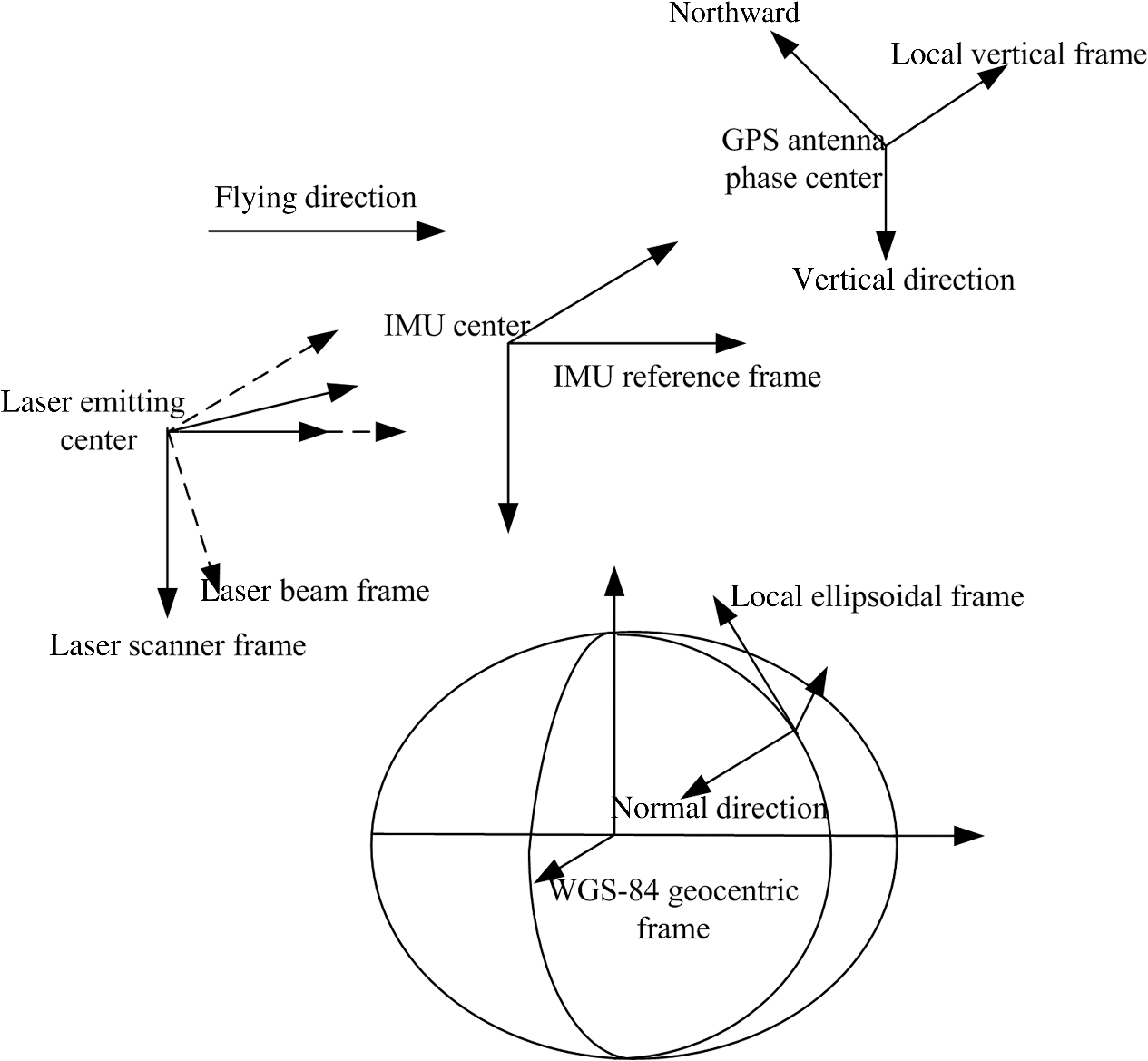
1. Introduction

Airborne light detection and ranging (LiDAR) is an active remote sensing technology for acquiring three-dimensional (3-D) information of the terrain effectively. Compared with conventional photogrammetry, LiDAR can provide 3-D information with higher accuracy and less production cost.¹^–³ Airborne LiDAR has been widely used in forestry and vegetation mapping, urban modeling, disaster mapping, archaeological survey, and geosciences. With the advance of technology, capabilities of airborne LiDAR systems have improved significantly. For example, the RIEGL LMS-Q1560 can be operated at a maximum pulse repletion rate of 800 kHz, and its range measurement accuracy reaches 20 mm at a range of 250 m.⁴ These improvements mean that the acquired laser points have much higher density and accuracy compared with earlier techniques. Airborne LiDAR consists of three systems: laser scanner, global positioning system (GPS), and inertial measurement unit (IMU). The raw observations, including the range to the target and scan angle measured by the scanner, as well as the position and orientation of the laser scanner measured by GPS and IMU, are used to calculate the coordinates of the discrete laser point using the direct georeferencing (DG) method.⁵ Because the DG method is sensitive to any source of systematic or random error,⁶^,⁷ the quality of airborne LiDAR data is easily contaminated, and discrepancies usually exist in overlapping areas of adjacent strips. It is essential to reduce or eliminate these systematic errors to guarantee the accuracy of LiDAR data. Modeling and analysis methods for airborne LiDAR systematic errors such as scan angle errors, range errors, and system component mount errors can be found in Schenk.⁸

Various methods have been proposed for eliminating the discrepancies in overlapping LiDAR strips. These methods can be divided into two categories. The first category makes the adjacent strips coincide by transforming point coordinates directly.⁹^–¹¹ Common transformations involve affine transformation and polynomial transformation. This kind of methods is not rigorous in view of the airborne LiDAR georeferencing mechanism, and it is difficult to compensate all the biases. The second category of methods, called system calibration, is based on the airborne LiDAR geolocation equation. It aims to determine the systematic error parameters and then use them in the geolocation equation to remove the error effects. The raw observations, such as range, scan angle, and position and attitude of the scanner should be provided for system calibration. Some systematic errors, such as scan angle error and range error, are consistent over time, but some others, such as bore-sight error, are more likely to change and should be calibrated for every mission. The point cloud accuracy is greatly dependent on the accuracy of system parameter calibration, and the calibration is a crucial procedure for airborne LiDAR data processing.

The primary procedure for system calibration is building the correspondence between the biased data and the reference data. Compared with images in conventional photogrammetry, it is difficult to identify tie points in overlapping LiDAR strips due to the irregular nature of the LiDAR points. Based on the high point density and short range associated with terrestrial LiDAR systems, Bang et al.¹² used the iterative closest point method to build the point-to-point correspondence between terrestrial and airborne LiDAR datasets, taking terrestrial LiDAR points as the reference to estimate the calibration parameters for the airborne LiDAR system. They also used the iterative closest patch (ICPatch) method to build the point-to-patch correspondence between the two datasets. The point-to-patch correspondence is indicative of the relationship between a point in the airborne LiDAR dataset and a triangular patch in the terrestrial LiDAR dataset derived from a triangulated irregular network generation procedure. Bang et al.¹² proposed a quasirigorous calibration procedure which requires time-tagged point cloud and trajectory position data. The ICPatch method was also used to build point–patch correspondence between two overlapping airborne LiDAR strips.¹³^–¹⁵

Planar features are most commonly used as conjugate features for airborne LiDAR system calibration. The conjugate planar patches cannot coincide together due to the systematic errors in the LiDAR system. Filin¹⁶ proposed a method using natural surfaces to identify bore-sight and range errors based on plane function. He concluded that moderate slopes with different orientations are sufficient for generating reliable results. Skaloud and Lichti¹⁷ used coplanar features for estimating bore-sight and range bias. Unlike other methods, they recovered the plane parameters together with the calibration parameters in a combined adjustment model. There were two datasets in their experiment; one was an urban dataset, which contains slopes with different inclinations and aspects, and the other was a dataset in a soccer field with a few horizontal or slightly inclined slopes. It turned out that calibration parameters obtained from the former dataset overmatched those obtained from the latter. The authors also pointed out that the range error correlates to the bore-sight angles and plane parameters. Hebel and Stilla¹⁸ employed an iterative combination of a random sample consensus-based robust estimation technique with a region growing approach to extract planar patches. They used planarity constraints for the bore-sight parameter calibration. Integrating terrestrial and airborne LiDAR data for system calibration, Bang et al.¹² used three correspondences (point-to-point, point-to-patch, and patch-to-patch), and found that the method using patch-to-patch correspondence had the most reliable results and was not sensitive to ill conditioned data like high random errors.

Although LiDAR system calibration based on coplanar constraints is feasible, there are some limitations which should be taken into account. The coplanar constraints can only ensure that the distance between the two patches is zero but cannot guarantee recovering them to the actual location. In most cases, the actual location of the reference plane is not available. In addition, the high correlation between different system errors may affect the calibration reliability. Most of these studies concluded that planar patches with different orientations are helpful in reducing the correlations between different system errors. Filin¹⁶ demonstrated that surfaces with positive and negative directions can reduce correlations between system parameters. Habib et al.¹⁹ illustrated the optimum configuration of planar patches which were orthogonal to the coordinate axes. These demands for planar patches reduce the practicality of the calibration method based on coplanar constraints because the number of patches with different aspects is limited in some calibration fields.

In this paper, we focus on the calibration of bore-sight angles because they can only be calibrated using an in-flight calibration procedure¹⁷ and have great influence on the quality of LiDAR data. We aim to find an optimal configuration of planar patches for airborne LiDAR system calibration. Such a configuration should be effective even though there is not a large amount of planar patches. It is beneficial to reduce the correlations between system errors and improve the reliability of the calibration results. This paper is organized as follows: In Sec. 2, we analyze the effects of bore-sight angles based on the laser point geolocation equation and propose an optimal configuration of the conjugate planar patches. In Sec. 3, the calibration method based on the coplanar constraints is provided. After describing the dataset in Sec. 4, we present the experiment and evaluate the effectiveness of the configuration of planar patches. In the end, we present our conclusions.

2. Principle of Bore-Sight Calibration

2.1.

Mathematical Model

As mentioned above, calibration of LiDAR system parameters is based on the laser point geolocation equation, which transforms the measurements to 3-D coordinates in the WGS84 geocentric reference frame. The form of the equation used in this paper is⁸^,²⁰

Eq. (1)

\vec{X} = R_{W} R_{G} R_{N} [R_{M} R_{L} [\begin{matrix} 0 \\ 0 \\ ρ \end{matrix}] + \vec{P}] + {\vec{X}}_{GPS},

where

\vec{X}

and

{\vec{X}}_{GPS}

are the vectors representing the position of the laser footprint and phase center of GPS receiver in the WGS-84 geocentric frame;

ρ

is the range between the laser firing point and the laser footprint;

\vec{P}

is the constant offset between the laser scanner and the phase center of the GPS receiver in the IMU reference frame;

R_{L}

is the rotation matrix from the laser beam frame to the laser scanner frame based on the scan angle;

R_{M}

is the rotation matrix from the laser scanner frame to the IMU reference frame;

R_{N}

represents the attitude matrix measured by IMU, transforming the IMU reference frame to the local vertical frame;

R_{G}

is the rotation matrix from the local vertical frame to the local ellipsoidal frame; and

R_{W}

is the rotation matrix from the local ellipsoidal frame to the WGS-84 geocentric frame and relates to longitude and latitude of the phase center of GPS receiver. The frame transform is illustrated in Fig. 1, and the definition of each frame is presented in Table 1. All frames are defined to be right-handed.

Fig. 1

Frame transform in laser point geolocation.

Table 1

Definitions of frames.

Frame	Definition
Laser beam frame	It originates at the laser emitting center. The $X$ -axis points to the flying direction and is perpendicular to the laser scanning plane. The $Z$ -axis points to the laser beam emitting direction.
Laser scanner frame	It is equal to the laser beam frame when the scan angle is zero.
IMU reference frame	It originates at the IMU reference center. The axes are approximately parallel to the axes of the laser scanner frame due to the mount errors.
Local vertical frame	It originates at the GPS antenna phase center. The $X$ -axis points northward, and the $Z$ -axis points vertically downwards.
Local ellipsoidal frame	It is similar to the local vertical frame. But the $Z$ -axis points to normal direction.
WGS-84 geocentric frame	It originates at the Earth’s center of mass. Its $Z$ -axis is the direction of the conventional terrestrial pole (CTP), as defined by BIH1984.0. The $X$ -axis points to the intersection of the zero meridian plane defined by the BIH1984.0 and the plane of the CTP’s equator.²¹

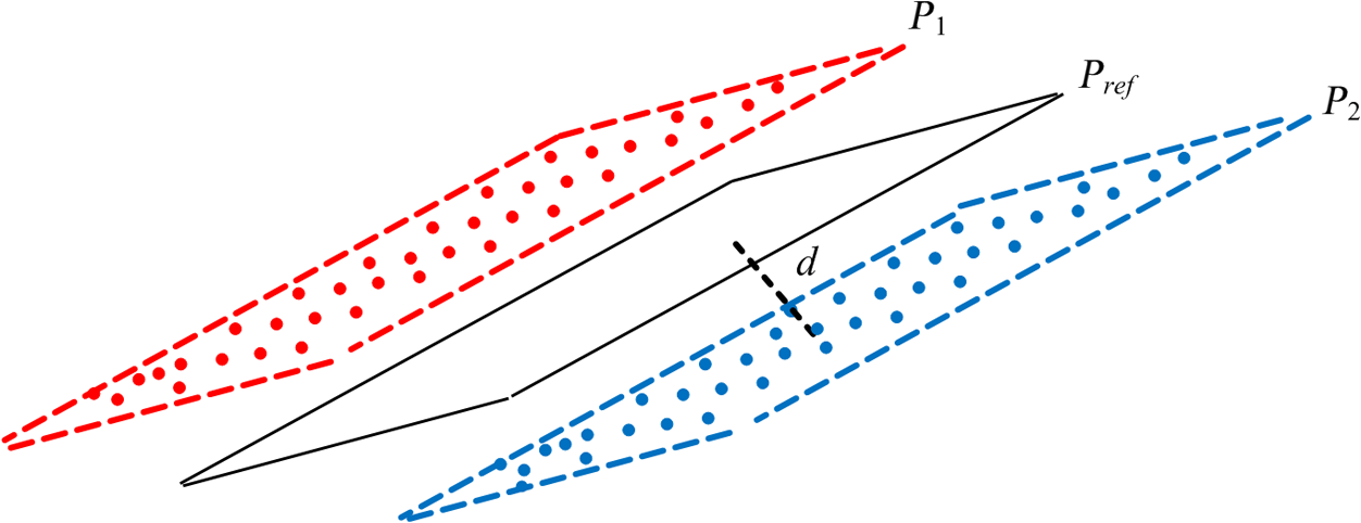
2.2.

Error Analysis

The bore-sight angles lead to discrepancies in overlapping areas. In order to reduce the correlations between the bore-sight angles and find an optimal configuration of the conjugate planar patches, it is essential to understand the effects of bore-sight angles. We assume that $α$ , $β$ , and $γ$ are the initial angles in rotation matrix $R_{M}$ , while $Δ α$ , $Δ β$ , and $Δ γ$ are the bore-sight angle errors in roll, pitch, and heading direction, respectively. Because the bore-sight angles are very small, the geolocation equation can be described as follows when considering the effects of bore-sight errors:

Eq. (2)

\vec{X} = R_{W} R_{G} R_{N} [Δ R_{M} R_{M} R_{L} [\begin{matrix} 0 \\ 0 \\ ρ \end{matrix}] + \vec{P}] + {\vec{X}}_{GPS},

where

Eq. (3)

R_{M} = [\begin{matrix} \cos γ & - \sin γ & 0 \\ \sin γ & \cos γ & 0 \\ 0 & 0 & 1 \end{matrix}] [\begin{matrix} \cos β & 0 & \sin β \\ 0 & 1 & 0 \\ - \sin β & 0 & \cos β \end{matrix}] [\begin{matrix} 1 & 0 & 0 \\ 0 & \cos α & - \sin α \\ 0 & \sin α & \cos α \end{matrix}],

Eq. (4)

Δ R_{M} = [\begin{array}{l} 1 & - Δ γ & Δ β \\ Δ γ & 1 & - Δ α \\ - Δ β & Δ α & 1 \end{array}] .

The bore-sight errors cause deviation of the target coordinates from the correct location. To better understand the error effects, we denote

R_{M}

as an identity matrix and analyze the coordinate bias in the IMU reference frame; therefore

R_{W}

,

R_{G}

,

R_{N}

,

\vec{P}

, and

{\vec{X}}_{GPS}

are not taken into account. The

x

,

y

, and

z

are the coordinates in the IMU reference frame, and

Δ x_{m}

,

Δ y_{m}

, and

Δ z_{m}

are the coordinate offsets between the true location and the biased location, which can be calculated by

Eq. (5)

[\begin{matrix} Δ x_{m} \\ y_{m} \\ Δ z_{m} \end{matrix}] = Δ R_{M} R_{M} R_{L} [\begin{matrix} 0 \\ 0 \\ ρ \end{matrix}] - R_{M} R_{L} [\begin{matrix} 0 \\ 0 \\ ρ \end{matrix}],

Eq. (6)

Δ x_{m} = Δ γ ρ \sin θ + Δ β ρ \cos θ Δ y_{m} = - Δ α ρ \cos θ Δ z_{m} = - Δ α ρ \sin θ,

where

θ

is the scan angle. If

Δ H = ρ \cos θ

represents the vertical distance from the scanner to the laser footprint, Eq. (6) can be changed to

Eq. (7)

Δ x_{m} = Δ γ Δ H \tan θ + Δ β Δ H Δ y_{m} = - Δ α Δ H Δ z_{m} = - Δ α Δ H \tan θ .

As shown in the above equations,

Δ α

generates offsets along both the

z

and

y

axes, while

Δ β

and

Δ γ

only generate offsets along the

x

axis. Therefore,

Δ α

is not related to

Δ β

or

Δ γ

in terms of coordinate offsets. The effect of

Δ β

relates to the flight altitude and is independent of the target distribution in the strip swath. Two strips with the same altitude but opposite directions lead to equal but opposite offsets caused by

Δ β

for the same target. The effects of

Δ α

and

Δ γ

relate to the scan angle. In a special case, when the target is at the nadir of the strip, the scan angle is zero, as are the effects of

Δ γ

and

Δ α

.

If $\vec{s} = {[s_{1} s_{2} s_{3} s_{4}]}^{T}$ represents the parameters of a plane, the plane equation is defined as

Eq. (8)

s_{1} x + s_{2} y + s_{3} z + s_{4} = 0 .

The distance between the actual plane and the biased point obtained by airborne LiDAR can be calculated as

Eq. (9)

d_{m} = \frac{(s_{1} Δ x_{m} + s_{2} Δ y_{m} + s_{3} Δ z_{m})}{\sqrt{s_{1}^{2} + s_{2}^{2} + s_{3}^{2}}} .

The

d_{m}

is equal to the dot product of the unit normal vector of the plane and the coordinate offset vector. Therefore, the distance is affected by plane parameters and coordinate offsets. This also explains why the planes with different orientations are beneficial to the reliability of bore-sight calibration. If the plane is parallel to the flight direction, the parameter

s_{1}

is zero. If the plane is horizontal, the parameters

s_{1}

and

s_{2}

are zero. In these special cases, the distance is only determined by

Δ α

. In addition, we can also use the distribution of conjugate patches to reduce the correlation between the bore-sight angles. For example, when an inclined planar patch is at the nadir of the strips and its normal vector is perpendicular to the

y

axis, if the actual plane parameters are provided,

Δ β

can be estimated accurately.

2.3.

Plane Parameter Estimation

The plane parameters are very important for bore-sight angle calibration based on conjugate planar patches. In most cases, the plane parameters are not available. The true position of planar patches, such as the roof of a gable building, is difficult to measure. Laying some specially designed targets²² facilitates the measurement but increases program costs. Without an accurate reference plane, the coplanar constraints can only keep the conjugate patches coinciding with each other but cannot guarantee relocating them to the actual position. Therefore, the calibration results may not be reliable even though the coplanar constraints are satisfied, especially when conjugate planar patches with different orientations are not enough.

For example, a gable-roof building is surveyed by two parallel strips with opposite directions. The roof ridge is perpendicular to the strips, and the building is located at the nadir of one strip and obliquely below the other strip. In Fig. 2, the solid black lines represent the true slopes of the roof. The red dotted lines represent the slopes obtained by the strip directly above the roof and are only affected by $Δ β$ bias because the scan angle is zero. The blue dotted lines represent the slopes obtained by the other strip and are affected by biases in $Δ α$ , $Δ β$ , and $Δ γ$ . If we just make $A_{1}$ and $A_{2}$ , $B_{1}$ and $B_{2}$ coplanar, respectively, but the true locations of A and B are not available, it does not guarantee that the biased planes will be fitted to the true locations or that the reliable bore sight angles will be obtained.

Fig. 2

Influence of bore-sight error on a gable roof building scanned by two parallel strips. 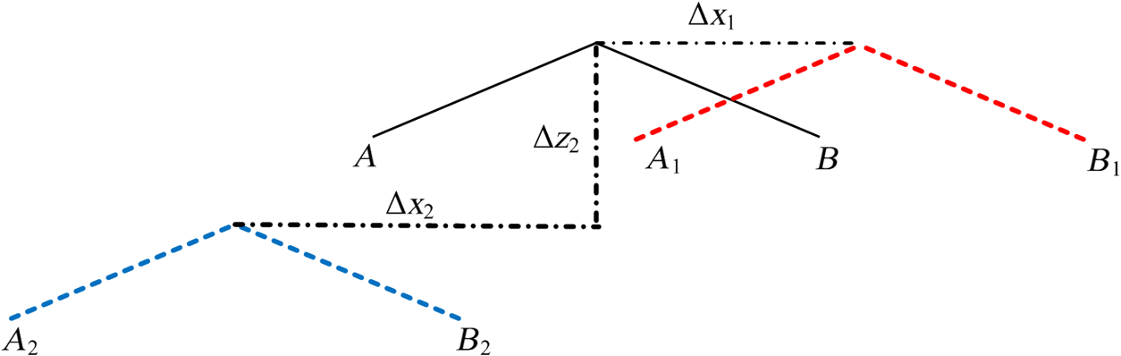$Δ x_{1}$ is the coordinate offset affected by $Δ β$ . $Δ x_{2}$ is the coordinate offset affected by $Δ β$ and $Δ γ$ . $Δ z_{2}$ is the coordinate offset affected by $Δ α$ .

An alternative approach is to fit plane parameters using appropriate laser points. If the conjugate planar surfaces scanned by different strips have symmetrical but opposite coordinate offsets affected by bore-sight angles, it is beneficial to use the biased points to fit a plane which is the same or similar to the plane in the true location. For example, a roof is surveyed by two opposite strips and at the nadir of the strips (Fig. 3). The measurements are only affected by $Δ β$ [see Eq. (7)]. The coordinate offsets are symmetrical, equal but opposite. The true location of the roof can be fitted accurately by the biased points and used as the reference to estimate $Δ β$ . Therefore, we can use the conjugate planar surfaces, satisfying the principle of symmetrical coordinate offsets to fit the plane parameters. These surfaces can be selected according to their distribution in the scanning swaths.

Fig. 3

Influence of bore-sight error on a gable roof building scanned by two strips with opposite directions. The solid black lines represent the true slopes of the roof. The red and blue dotted lines represent the slopes obtained by two strips respectively.

2.4.

Optimal Configuration of Conjugate Planar Patches

As demonstrated in previous studies, planar patches with different aspects increase the quality of bore-sight angle calibration.¹⁶^,¹⁷^,¹⁹ If we use fewer planar patches, the distribution of the planar patches should be considered. According to the above analyses, there are some principles regarding the optimal configuration of conjugate planar patches. The first is the symmetry of the bore-sight angles effects, meaning the coordinate offsets of conjugate planes caused by bore-sight angles should be equal but opposite. The actual plane parameters can be fitted approximately by the biased laser points and taken as the reference plane. The second principle is low correlations between the bore-sight angles. It is better to choose the patch scanned by one strip which is affected only by one or two of the three bore-sight angles. For example, the planar patch located at the nadir of one strip is not affected by $Δ γ$ . It is useful to reduce the correlation between $Δ β$ and $Δ γ$ . We will validate the two principles in our experiments.

3. Method

3.1.

Data Preprocessing

The data preprocessing procedure aims to extract and match corresponding features. First, we calculate the laser point coordinates using the observed values, such as the scan angle, the distance between the sensor and the target, and the position and attitude of the sensor based on the geolocation equation. Then we manually identify the corresponding surfaces. Although there are many approaches that can be used to extract the roof surfaces automatically, manual extraction is a simple way to select a small number of planes based on the principles of symmetry and low correlation. We choose roof surfaces with different aspects and distributions to decouple the bore-sight angles. Some noise points, such as the bumps on the roof surface, should be removed. Through the data preprocessing procedure, a number of corresponding planes and observed values of laser points are prepared for bore-sight calibration.

3.2.

Bore-Sight Calibration

Due to the systematic errors, the conjugate surfaces in the overlapping strips do not coincide with one another. Therefore, the calibration procedure uses the coplanarity of conjugate planes as the constraint conditions to recover the system parameters. When the systematic errors are eliminated, all the conjugate surfaces are recovered to their true locations. Because the parameters of the true surface are not known, all the LiDAR points belonging to the same roof plane are used to fit a reference surface $P_{ref}$ based on the least square fitting method. Figure 4 shows a pair of conjugate planar patches scanned by two strips and the fitted reference plane. The distance $d$ between a point and $P_{ref}$ can be described as

Eq. (10)

d = \frac{(s_{1} x + s_{2} y + s_{3} z + s_{4})}{\sqrt{s_{1}^{2} + s_{2}^{2} + s_{3}^{2}}},

where

s_{1 - 4}

are parameters of the reference plane.

Fig. 4

A pair of conjugate planar patches and the reference plane fitted by the biased points.

The roof plane is usually rough, and not all the distances are zeros. The right side of Eq. (10) can be expanded by the Taylor function, so the normal equation is

Eq. (11)

V = B X + L,

where

V

is the residual of the distance matrix,

B

is the coefficient matrix,

L

is the distance matrix, and

X

is the column vector of

Δ α

,

Δ β

, and

Δ γ

. According to the least squares adjustment solution, the parameters can be estimated when the sum of the weighted square of the residuals is minimized, such that

Eq. (12)

X = - {(B^{T} P B)}^{- 1} B^{T} P L,

where

P

is the weight matrix and is usually assumed to be an identity matrix. At the beginning,

α

,

β

,

γ

,

Δ α

,

Δ β

, and

Δ γ

are set to zero. When

Δ α

,

Δ β

, and

Δ γ

are calculated,

α

,

β

, and

γ

are added to

Δ α

,

Δ β

, and

Δ γ

, respectively, for the next iteration. After a few iterations,

Δ α

,

Δ β

, and

Δ γ

are close to zero. The iterative procedure runs until

Δ α

,

Δ β

, and

Δ γ

are small enough or the iterations exceed the threshold value. In the end,

α

,

β

, and

γ

are the value of bore-sight angles.

4. Dataset Description

The data used in this experiment were acquired in Gansu province, China, in 2014. The laser scanner is a RIEGL Q780 whose maximum pulse repetition frequency (PRF) is 400 kHz. The wavelength is 1064 ns, the laser beam divergence is 0.25 mrad, and the field of view is 60 deg.⁴ The Applanix POS AV 610 was used to measure the position and attitude of the laser scanner. The dataset consists of six strips, as shown in Fig. 5, which were captured with a PRF of 400 kHz and a scan frequency of $102 lines / s$ . The density of the point cloud is about $5.5 points / m^{2}$ , and the flying altitude is 900 m above ground level. The average ground speed of the plane is $160 km / h$ . The overlap ratio of neighboring strips is about 60% to guarantee that more targets can be scanned from different aspects.

Fig. 5

Top view of the six strips used for calibration. B1–B4 are gable roof buildings used for bore-sight calibration. The red arrows represent flying directions.

The raw data was processed by the RiANALYZE software and the POSPac MMS software. The RiANALYZE software was used to decompose the full wave data recorded by the laser scanner to obtain the range and scan angle for each target. The result was stored in a data file with a .sdc suffix, including the range, GPS time, amplitude, laser point coordinates in the laser body frame, and so on. The POSPac MMS software, a global navigation satellite system inertial processing software for airborne application, is used to process the raw GPS and IMU data to calculate the accurate position and attitude of the scanner for each corresponding GPS time and store the result in a data file with a. sbet suffix. The postprocessing errors are 0.0025 deg for roll and pitch, 0.005 deg for the heading, 0.05 m for the horizontal position, and 0.1 m for the vertical position.²³ The raw observations of each point, such as range, scan angle, and position and attitude of the scanner, can be extracted from these files and used for bore-sight calibration according to the method introduced in Sec. 3.

Four gable roof buildings are utilized for bore-sight calibration as illustrated in Fig. 6. The buildings are observed by multiple strips with different scan angles. Table 2 describes the relationship between the buildings and scanning strips. In addition, the conjugate planes have different orientations in order to decouple the correlation between bore-sight angles. B2 and B3 are scanned by three parallel strips. They are located at the center of the swath of one strip and at the margin of the other two. Their distribution conforms to the principles of symmetry and low correlation. The data provider supplied the bore-sight angles calibrated by RiProcess software, which can be used as reference values.

Fig. 6

Top view of gable roof buildings. The buildings labeled by yellow rectangles in (a)–(d) are buildings B1–B4 in sequence.

Table 2

Building and strips.

Gable roof building	Strip
B1	2,3,5,6
B2	4,5,6
B3	4,5,6
B4	2,3,4

5. Experiment and Discussion

5.1.

Validation of Planar Patches Configuration

According to the analysis in Sec. 2, the orientation and distribution of planar patches have influences on the calibration of bore-sight angles. In order to analyze the influences, seven conjugate plane configurations are designed to compare the accuracy of the results. The first three configurations are used to validate the effect of different plane orientations. Configurations IV, V, and VI are used to validate the effect of the principles of symmetry and low correlation mentioned in Sec. 2.4. The last configuration uses all the planes acquired by the strips. Table 3 displays the buildings and scanning strips used in each configuration.

Table 3

Buildings and scanning strips used in each configuration.

Configuration	Gable roof building	Scanning strips
I	B1	5,6
II	B1,B2	5,6
III	B1	2,3,5,6
	B2	5,6
	B3	5,6
	B4	1,2,3
IV	B2	4,5,6
V	B3	4,5,6
VI	B2,B3	4,5,6
VII	all	All

The proposed method was applied to the datasets described above. Table 4 is an overview of the bore-sight calibration results of each configuration. The results of the last four configurations are similar to the values calculated by the RiProcess software.

Table 4

Result of bore-sight calibration.

Configuration	α (deg)	β (deg)	γ (deg)	Number of iterations
I	$- 0.0141$	0.0545	$- 0.0079$	6
II	$- 0.0206$	0.0420	$- 0.044$	20
III	$- 0.0243$	0.0644	0.0362	15
IV	$- 0.0231$	0.0744	0.0591	6
V	$- 0.0218$	0.0669	0.0495	4
VI	$- 0.0211$	0.0688	0.0523	4
VII	$- 0.0214$	0.0682	0.0533	5
RiProcess	$- 0.0203$	0.0690	0.0536	—

In configuration I, two roof planes are used to estimate the bore-sight angles. After six iterations, the discrepancies between the roof planes of B1 scanned by strips 5 and 6 are eliminated, as illustrated in Fig. 7. However, the estimated bore-sight angles are incorrect. The distance from the point calibrated by the results of configuration I to the corresponding point calibrated by the RiProcess software is more than 20 cm (Fig. 8). The biased points are not recovered to their actual positions. This proves that two planar patches without actual reference plane parameters cannot achieve reliable bore-sight angles even though the coplanar constraints are satisfied. Therefore, more planes with different orientations are needed.

Fig. 7

(a) Profile of B1 before calibration. (b) Profile of B1 after calibration. The blue and red points are obtained by strip 5 and strip 6, respectively.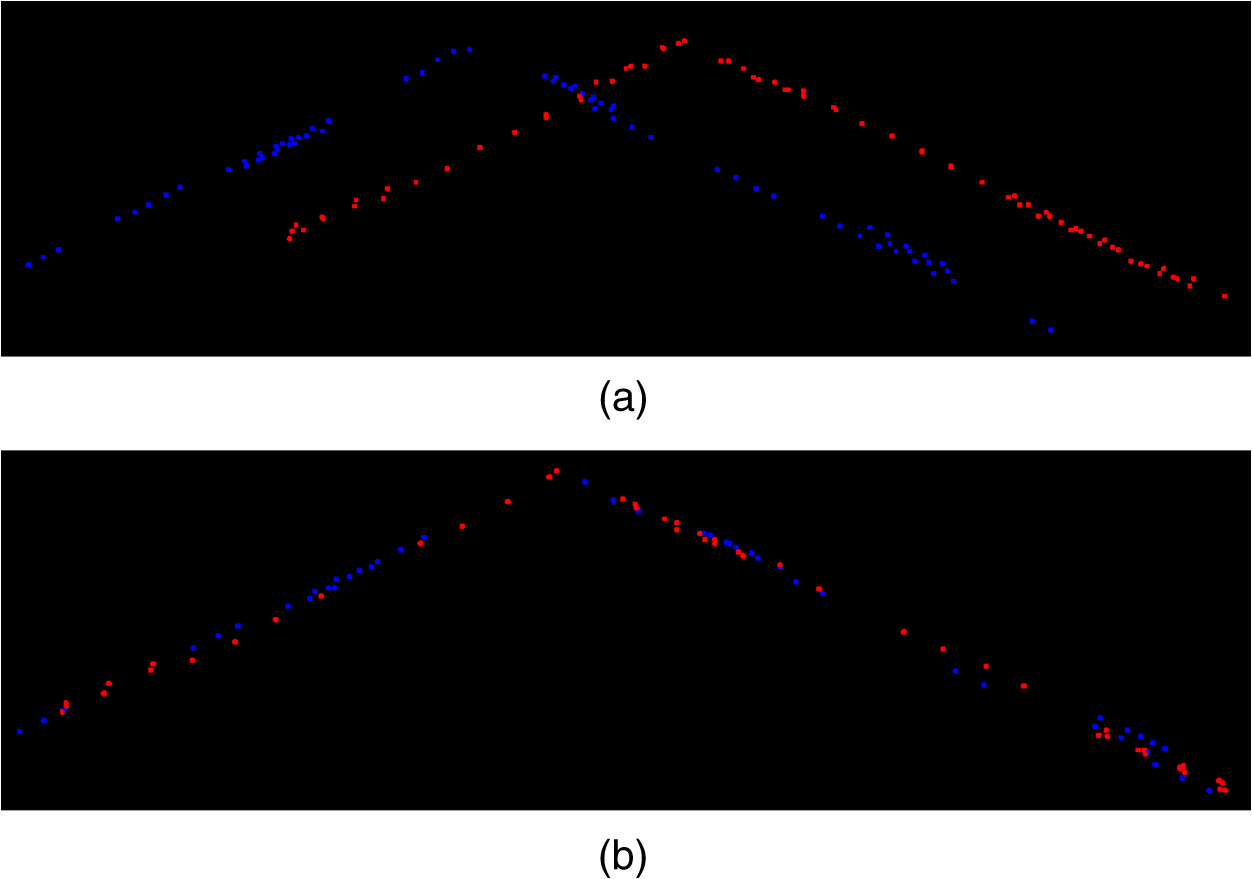

Fig. 8

(a) Profile of B1. (b) Top view of B1. The blue points represent the calibrated points using the results of configuration I, and the red points represent the calibrated points using the results of RiProcess.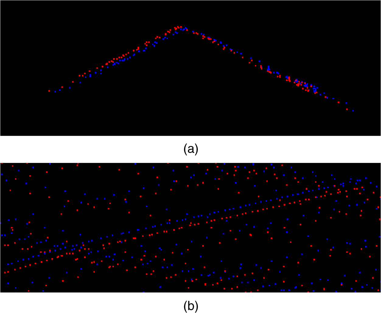

More planar patches are used in configurations II and III. In configuration II, $Δ β$ and $Δ γ$ do not converge after 20 iterations. In configuration III, $Δ α$ and $Δ β$ are close to the RiProcess results, but $Δ γ$ is remarkably different. The reliability of the bore-sight angle estimation can be increased by using more planar patches, but the exact amount of planar patches needed is difficult to determine.

The results of configurations IV, V, and VI are homologous to the RiProcess results. Though, there are just two planar patches of one gable roof building in configurations IV and V, they are covered by three strips and satisfy the principles of symmetry and low correlation. The patches of configuration VI are the combination of the patches in configurations IV and V. The experiment results demonstrate that these configurations are beneficial to the bore-sight calibration. Configuration V is used here as an example for analysis. In order to analyze the error effects easily, we analyze the errors in the IMU reference frame as explained in Sec. 2.2. The ridge of the gable building B3 is parallel to the flight direction, so the coordinate offset along the $y$ axis caused by $Δ α$ is zero. Strips 4 and 6 are parallel and have the same direction. B3 is located obliquely below the two strips and scanned by opposite scan angles. Comparing the laser point coordinate offsets of B3 obtained by strips 4 and 6 according to Eq. (7), both the offsets along the $Z$ axis caused by $Δ α$ and the offsets along the $x$ axis caused by $Δ γ$ are opposite, while the offsets along the $x$ axis caused by $Δ β$ are equal. B3 is at the nadir of strip 5, so the scan angle is zero and the effects of $Δ α$ and $Δ γ$ do not need to be taken into account. Because the flight direction of strip 5 is opposite to that of strips 4 and 6, the coordinate offsets along the $x$ axis caused by $Δ β$ of the laser points obtained by strip 5 are opposite to that of laser points obtained by strips 4 and 6. The profiles of the biased roof obtained by strips 4, 5, and 6 can be seen in Fig. 9. The actual roof can be fitted approximately by these biased points through a few iterations. The experiments prove that conjugate planar patches that satisfy the principles of symmetry and low correlation are beneficial to the reliability of bore-sight angle calibration.

Fig. 9

Profiles of gable building B3. A and B are two planar patches of B3 representing the actual location. The other dot lines represent the biased patches obtained by strips 4, 5, and 6.

The data used in configuration VII add roof planes of B2 and B3 scanned by strips 4, 5, and 6 to the data used in configuration III. The number of iterations is reduced to 4, and the estimated bore-sight angles are very close to the results of RiProcess with a deviation of about 0.001 deg. Additionally, the correlation matrices of unknown parameters for Configuration III and VII are shown in Table 5. The appropriate configuration greatly decreases the correlations between bore-sight angles.

Table 5

Correlation matrices for configuration III and VII.

	Configuration III			Configuration VII
	Δα	Δβ	Δγ	Δα	Δβ	Δγ
$Δ α$	1.00	$- 0.21$	$- 0.20$	1.00	$- 0.13$	$- 0.12$
$Δ β$	$- 0.21$	1.00	0.84	$- 0.13$	1.00	0.30
$Δ γ$	$- 0.20$	0.84	1.00	$- 0.12$	0.30	1.00

5.2.

Effects of Reference Plane Parameters

The coordinate offsets of the conjugate planar patches in the first configuration are not symmetrical, and the reference plane fitted by the biased points is not close to the actual location. The calibration procedure does not recover the laser points to the actual positions. In order to validate the effects of the reference plane parameters, we fit the plane parameters using laser points calibrated by the RiProcess software and apply them to configurations I, II, and III. The new results of these configurations are listed in Table 6.

Table 6

Result of bore-sight calibration.

Configuration	α (deg)	β (deg)	γ (deg)	Number of iterations
I	$- 0.0254$	0.0683	0.0672	2
II	$- 0.0218$	0.0721	0.0647	2
III	$- 0.0223$	0.0678	0.0542	2
RiProcess	$- 0.0203$	0.0690	0.0536	—

The results show major improvements for the estimation of bore-sight angles compared with the results using the parameters fitted by biased points. Moreover, only two iterations are needed. Accurate reference parameters play an important role in the calibration procedure.

5.3.

Representative Points

In the above experiments, all laser points of the roof planar patches are used to build error equations. Each point builds one error equation, resulting in a very large set of error equations. The roof patches are relatively limited in size, and there are only minor differences in the observation values of neighboring points, such as scan angle, range, and attitude of scanner. Since the bore-sight angle effects on the points of one roof patch obtained by the strip are similar, we select some representative points to build the error equation.

The laser points of a roof patch obtained by one strip can be used to fit a plane, and the distance from each point to the plane can be calculated. The nearest points to the plane are chosen to represent this patch and used to build the error equations. We select representative points for the planar patches in configuration VII according to the distance. All the distances can be regarded as a Gaussian distribution (Fig. 10), with an σ value of 0.0333 m. The calibration results and the number of error equations are shown in Table 7.

Fig. 10

A Gaussian distribution of distances between laser points and reference planes. The horizontal and vertical axes are the distance and number of points, respectively.

Table 7

Result of bore-sight calibration by representative points.

	α (deg)	β (deg)	γ (deg)	Number of error equations	Calculation time (sec)	Number of iterations
$d < 0.0001$	$- 0.0222$	0.0700	0.0570	95	2.94	6
$d < 0.001$	$- 0.0220$	0.0695	0.0585	985	3.11	6
$d < 0.01$	$- 0.0215$	0.0688	0.0593	9571	5.20	5
$d < 0.03$	$- 0.0215$	0.0686	0.0582	24452	8.16	5
$d < 0.07$	$- 0.0215$	0.0683	0.0542	35594	10.56	5
$d < 0.1$	$- 0.0215$	0.0682	0.0532	36966	10.73	5
$d < 0.15$	$- 0.0214$	0.0682	0.0533	37135	11.16	5

The calibration procedure with less representative points consumed less time but also obtained less accurate results. When the distance limit is 0.07 m (about $2 σ$ ), more than 95% of the points are used and the results are close to the RiProcess results. The changes in $α$ and $β$ are less than 0.002 deg, which is smaller than the postprocessing roll and pitch accuracy of POS. The change in $γ$ is about 0.006 deg, which is greater than the postprocessing heading accuracy of POS. According to Eq. (7), the 0.006 deg Δγ causes a coordinate offset of 6 cm along the flight direction when the flight altitude is 1000 m and the scan angle is 30 deg. Therefore, it is better to use more points to eliminate the effects of other random errors. An alternative method is to use fewer representative points to get the initial values of bore-sight angles and then use more points to improve the accuracy, but this alternative method does not greatly improve efficiency.

5.4.

Coincidence Validation

In the above sections, the bore-sight angles calculated by RiProcess were taken as reference to evaluate the reliability of our experiment results. We also checked the coincidence of conjugate planar patches by the profile. In this section, we calculate the standard deviation of the distances from laser points to the reference plane to evaluate the calibration quality. For a roof planar patch scanned by multiple strips, we fit the reference plane with the points obtained by all strips and calculate the distance to the reference plane for every point. We then calculate the standard deviation of the distances. Comparing the standard deviation by using points before and after calibration can indicate the improvements of plane alignment as visualized in Figs. 11(a) and 11(b). We calculate the standard deviations of distances for the points calibrated by the bore-sight results of RiProcess and configurations VI and VII in Sec. 5.1 to compare their accuracy.

Fig. 11

Distance from laser point to the reference plane. Red and blue points are laser points scanned by different strips. Pref is the reference plane fitted by the points. (a) Distances calculated by points before calibration; (b) distances calculated by points after calibration; (c) distances calculated by every single strip to compute roughness of the roof plane.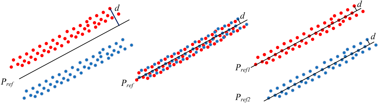

If the roof planar patch is an absolute plane, and the conjugate patches coincide completely, all the distances should be zero. However, the roof planar patch is rugged, so the standard deviation of the distances is influenced not only by the coincidence of the conjugate planar patches but also by the roof roughness as shown in Fig. 11(b). We calculate another standard deviation which represents the roughness of the roof. The procedure differs in that we fit the plane separately with the biased points obtained by every single strip and calculate the distances from the points to the corresponding plane, then calculate the standard deviation for all the distances. We use the biased points because we assume the bore-sight angle errors affect the roof positions but lead to little deformation. If the standard deviation calculated by the calibrated points is close to the standard deviation representing the roughness, it proves that the calibrated patches coincide well and the estimated bore-sight angles are reliable.

As shown in Table 8, the standard deviations of distances for the points calibrated by the bore-sight results of RiProcess and configurations VI and VII are similar, and all of them are much smaller than the standard deviation before calibration. This proves that the bore-sight calibration improves the coincidence of conjugate planes greatly. However, all the standard deviations of the three groups of distances are greater than the standard deviation representing the roughness. The average increase is approximately 2 cm, and the largest is 4 cm. This indicates that some residual discrepancies still exist and may be ascribed to other errors, such as GPS position errors and range errors.

Table 8

Standard deviation of distances.

Building	Roof planar patch	Std (roughness)	Std (before calibration)	Std (configuration VI)	Std (configuration VII)	Std (RiProcess)
B1	P1	0.032	0.260	0.047	0.046	0.046
B1	P2	0.027	0.220	0.052	0.050	0.051
B2	P1	0.032	0.259	0.053	0.049	0.049
B2	P2	0.031	0.286	0.067	0.071	0.071
B3	P1	0.040	0.338	0.067	0.064	0.064
B3	P2	0.037	0.343	0.056	0.059	0.059
B4	P1	0.025	0.115	0.046	0.046	0.046
B4	P2	0.039	0.152	0.051	0.050	0.050

6. Conclusions

Bore-sight angle errors lead to discrepancies in the overlapping strips which degrade the accuracy of airborne LiDAR data and affect subsequent applications. In this paper, we propose an improved method for bore-sight calibration based on the principles of symmetry of coordinate offsets and low correlations between bore-sight angles. Though many researchers have discussed bore-sight self-calibration using conjugate planer patches, they emphasize using patches with different orientations to decrease the correlations between the bore-sight angles. Therefore, a large number of patches are needed to guarantee the reliability of calibration results. In our experiment, two gable roof buildings scanned by three strips in configuration VI were used for bore-sight calibration, and the estimated parameters were approximate to the results calculated by the RiProcess software. Compared with previous studies, our study has the following contributions:

1. The optimal configuration of planar patches based on the principles of symmetry of coordinate offsets and low correlations requires only a few patches. It is easier to find an appropriate calibration field. It also can decrease the correlations between bore-sight angles and increase the reliability of the results.
2. The control information of the reference plane is not needed. The reference plane parameters can be fitted by biased points because the coordinate offsets of conjugate patches are symmetrical and the fitted parameters are approximate to the actual ones by iteration.
3. The optimal configuration of planar patches improves the calculation efficiency because it uses a few patches. We tried to use representative points to improve the calculation efficiency when more patches are added, but the accuracy of the results decreased.
4. It provides a good instruction for making a flight plan for bore-sight calibration. Especially when there are not a great number of planar patches in the calibration field, it is very useful for designing the strips according to the optical configuration.
5. The optimal configuration is also applicable for eliminating discrepancies in the overlapping areas using transformation models for some end users who only get the point data set without original observation values. The configuration of planar patches is also an important factor affecting the reliability of transform parameters.

The configuration of conjugate planar patches based on the principles of symmetry of coordinate offsets and low correlations is a major improvement for bore-sight angle calibration. Further research will concentrate on the calibration of other systematic errors, such as the scan angle error and range error, as well as how to decrease the correlations between these errors and improve the reliability of calibration results.

Acknowledgments

The authors would like to thank Xia Meng, Yue Zhao, and Sichong Chen, who provided the research data and technical services. The research was funded by the National Natural Science Foundation of China (No. 91125003).

References

1.

F. Ackermann, “Airborne laser scanning—present status and future expectations,” ISPRS J. Photogramm., 54 (2), 64 –67 (1999). http://dx.doi.org/10.1016/S0924-2716(99)00009-X IRSEE9 0924-2716 Google Scholar

2.

J. C. McGlone et al., Manual of Photogrammetry, 5th ed.American Society for Photogrammetry and Remote Sensing, Bethesda, Maryland (2004). Google Scholar

3.

N. El-Sheimy, C. Valeo and A. Habib, Digital Terrain Modeling: Acquisition, Manipulation, and Applications, 1st ed.Artech House, Norwood, Massachusetts (2005). Google Scholar

4.

, “LMS-Q1560 Datasheet,” http://www.riegl.com/uploads/tx_pxpriegldownloads/DataSheet_LMS-Q1560_2015-03-19.pdf Google Scholar

5.

J. Skaloud, “Direct georeferencing in aerial photogrammetric mapping,” Photogramm. Eng. Rem. S., 68 (3), 207 –210 (2002). Google Scholar

6.

N. Yastikli and K. Jacobsen, “Direct sensor orientation for large scale mapping—potential, problems, solutions,” Photogramm. Rec., 20 (111), 274 –284 (2005). http://dx.doi.org/10.1111/j.1477-9730.2005.00318.x PGREAY 0031-868X Google Scholar

7.

N. Yastikli and K. Jacobsen, “Influence of system calibration on direct sensor orientation,” Photogramm. Eng. Rem. S., 71 (5), 629 –633 (2005). http://dx.doi.org/10.14358/PERS.71.5.629 Google Scholar

8.

T. Schenk, “Modeling and analyzing systematic errors in airborne laser scanners,” Tech. Notes Photogramm., 19 42 (2001). Google Scholar

9.

J. Lee et al., “Adjustment of discrepancies between LIDAR data strips using linear features,” IEEE Geosci. Remote Sens. Lett., 4 (3), 475 –479 (2007). http://dx.doi.org/10.1109/LGRS.2007.898079 Google Scholar

10.

A. Habib et al., “LiDAR strip adjustment using conjugate linear features in overlapping strips,” in Proc. Int. Archives of the Photogrammetry, Remote Sensing and Spatial Information Sciences, 385 –390 (2008). Google Scholar

11.

M. Rentsch and P. Krzystek, “LiDAR strip adjustment using automatically reconstructed roof shapes,” in Proc. Int. Archives of the Photogrammetry, Remote Sensing and Spatial Information Sciences, 158 –164 (2009). Google Scholar

12.

K. I. Bang et al., “Integration of terrestrial and airborne LiDAR data for system calibration,” in Proc. Int. Archives of the Photogrammetry, Remote Sensing and Spatial Information Sciences, 391 –398 (2008). Google Scholar

13.

K. I. Bang, A. Habib and A. Kersting, “Estimation of biases in lidar system calibration parameters using overlapping strips,” Can. J. Remote Sens., 36 (2), S335 –S354 (2010). http://dx.doi.org/10.5589/m10-054 CJRSDP 0703-8992 Google Scholar

14.

A. F. Habib et al., “Geometric calibration and radiometric correction of LiDAR data and their impact on the quality of derived products,” Sensors, 11 (9), 9069 –9097 (2011). http://dx.doi.org/10.3390/s110909069 SNSRES 0746-9462 Google Scholar

15.

A. Habib et al., “Alternative methodologies for LiDAR system calibration,” Remote Sens., 2 (3), 874 –907 (2010). http://dx.doi.org/10.3390/rs2030874 Google Scholar

16.

S. Filin, “Recovery of systematic biases in laser altimetry data using natural surfaces,” Photogramm. Eng. Rem. S., 69 (11), 1235 –1242 (2003). http://dx.doi.org/10.14358/PERS.69.11.1235 Google Scholar

17.

J. Skaloud and D. Lichti, “Rigorous approach to bore-sight self-calibration in airborne laser scanning,” ISPRS J. Photogramm., 61 (1), 47 –59 (2006). http://dx.doi.org/10.1016/j.isprsjprs.2006.07.003 IRSEE9 0924-2716 Google Scholar

18.

M. Hebel and U. Stilla, “Simultaneous calibration of ALS systems and alignment of multiview LiDAR scans of urban areas,” IEEE Trans. Geosci. Remote Sens., 50 (6), 2364 –2379 (2012). http://dx.doi.org/10.1109/TGRS.2011.2171974 IGRSD2 0196-2892 Google Scholar

19.

F. Habib et al., “LiDAR system self-calibration using planar patches from photogrammetric data,” in The 5th Int. Symp. Mobile Mapping Technology, (2007). Google Scholar

20.

C. Vaughn et al., “Georeferencing of airborne laser altimeter measurements,” Int. J. Rem. Sens., 17 (11), 2185 –2200 (1996). http://dx.doi.org/10.1080/01431169608948765 IJSEDK 0143-1161 Google Scholar

21.

Z. Lu, Q. Yunying and S. Qiao, Geodesh: Introduction to Geodetic Datum Geodetic Systems, Springer-Verlag, Berlin Heidelberg (2014). Google Scholar

22.

N. Csanyi and C. K. Toth, “Improvement of lidar data accuracy using lidar-specific ground targets,” Photogramm. Eng. Rem. S., 73 (4), 385 –396 (2007). http://dx.doi.org/10.14358/PERS.73.4.385 Google Scholar

23.

, “POSAV specifications,” (2012) http://www.applanix.com/media/downloads/products/specs/posav_specs_1212.pdf Google Scholar

Biography

Dong Li received his MS degree in GIS from the School of Remote Sensing and Information Engineering, Wuhan University, 2006. Currently, he is pursuing his PhD at the University of Chinese Academy of Sciences and working at the Institute of Remote Sensing and Digital Earth, Chinese Academy of Sciences. His research mainly focuses on LiDAR data processing and application.

Huadong Guo graduated from the Geology Department at Nanjing University in 1977 and received his MS degree from the Graduate University of the Chinese Academy of Science in 1981. He is a professor with the Institute of Remote Sensing and Digital Earth, Chinese Academy of Sciences, Beijing, China. His current research includes radar remote sensing, applications of earth observing technologies to global change, and digital earth.

Cheng Wang received his PhD degree in remote sensing from Université Louis Pasteur, Strasbourg, France in 2005. He is currently a professor with the Institute of Remote Sensing and Digital Earth, Chinese Academy of Sciences, Beijing, China. His research interests include light detection and ranging and remote sensing for ecology and digital heritage applications.

Pinliang Dong received his PhD in geology from the University of New Brunswick, Canada, in 2003. He is an associate professor at the Department of Geography and the Environment, University of North Texas (UNT), Denton, Texas, USA. His research interests include remote sensing, geographic information systems (GIS), digital image analysis, and LiDAR applications in forestry, urban studies, and geosciences.

Zhengli Zuo received his BS degree in photogrammetry and remote sensing from Wuhan Technical University of Surveying and Mapping in 1987. He is a senior engineer with the Institute of Remote Sensing and Digital Earth, Chinese Academy of Sciences, Beijing, China. His research interests include airborne remote sensing data acquisition and application

CC BY: © The Authors. Published by SPIE under a Creative Commons Attribution 4.0 Unported License. Distribution or reproduction of this work in whole or in part requires full attribution of the original publication, including its DOI.

Citation Download Citation

Dong Li, Huadong Guo, Cheng Wang, Pinliang Dong, and Zhengli Zuo "Improved bore-sight calibration for airborne light detection and ranging using planar patches," Journal of Applied Remote Sensing 10(2), 024001 (9 May 2016). https://doi.org/10.1117/1.JRS.10.024001

Published: 9 May 2016

Access the abstract

JOURNAL ARTICLE
17 PAGES

DOWNLOAD PAPER SAVE TO MY LIBRARY

GET CITATION

CITATIONS

Cited by 5 scholarly publications.

Explore citations on Lens.org

KEYWORDS

Calibration

LIDAR

Buildings

Global Positioning System

Reliability

Laser scanners

Error analysis

1.

Introduction

2.

Principle of Bore-Sight Calibration

2.1.

Mathematical Model

Eq. (1)

Fig. 1

Table 1

2.2.

Error Analysis

Eq. (2)

Eq. (3)

Eq. (4)

Eq. (5)

Eq. (6)

Eq. (7)

Eq. (8)

Eq. (9)

2.3.

Plane Parameter Estimation

Fig. 2

Fig. 3

2.4.

Optimal Configuration of Conjugate Planar Patches

3.

Method

3.1.

Data Preprocessing

3.2.

Bore-Sight Calibration

Eq. (10)

Fig. 4

Eq. (11)

Eq. (12)

4.

Dataset Description

Fig. 5

Fig. 6

Table 2

5.

Experiment and Discussion

5.1.

Validation of Planar Patches Configuration

Table 3

Table 4

Fig. 7

Fig. 8

Fig. 9

Table 5

5.2.

Effects of Reference Plane Parameters

Table 6

5.3.

Representative Points

Fig. 10

Table 7

5.4.

Coincidence Validation

Fig. 11

Table 8

6.

Conclusions

Acknowledgments

References

Biography

Show All Keywords

Keywords/Phrases

Search In:

Publication Years