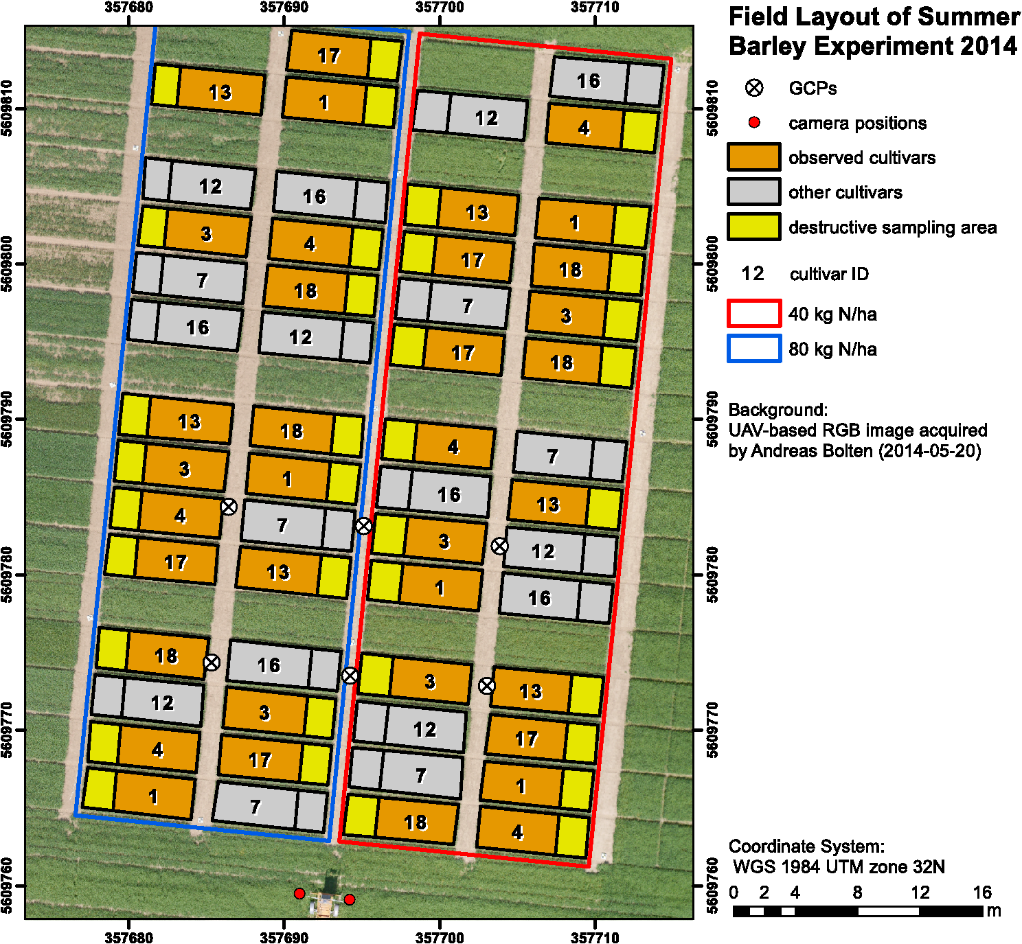
1.

Introduction

Monitoring growth, vitality, and stress of crops is a key task in precision agriculture.¹ This can be realized by nondestructive monitoring of structural crop parameters such as plant height and growth as well as by monitoring physiological parameters such as chlorophyll or water content. The structural parameters can be monitored using crop surface models (CSMs)^2–4 and have been used for biomass estimation on the field level,^5,6 while monitoring of physiological parameters is made possible by multi- and hyperspectral or microwave sensors.^7–11 Combined approaches using the synergies that structural and physiological crop parameter sensing provide have successfully been investigated.^6,–14 In general, remote sensing-based crop monitoring is a very wide research field. A large variety of sensor types are used across different scale levels to benefit precision agriculture.¹ These sensors are used from spaceborne, airborne, and terrestrial platforms.

The generation of multitemporal CSMs is an analysis approach made possible by the different technologies that allow the retrieval of very high resolution three-dimensional (3-D) data. CSMs are 3-D (more precisely 2.5-D, because only one $z$ value is stored per $x/y$ coordinate pair) raster representations of crop canopies. The concept of CSMs has been introduced by Hoffmeister et al.¹⁵ for the multitemporal monitoring of crop growth patterns on a field scale across phenological stages using light detection and ranging (LiDAR) data. The crop growth between dates can be derived by subtracting the plant height of successive dates. CSMs have not only been derived from LiDAR data^4,16,17 but also from airborne red, green, blue (RGB) imagery.^2,5,13 Hyperspectral CSMs have also been derived from hyperspectral snapshot cameras.¹⁸

LiDAR is a technology that allows the detection of object points in 3-D space by measuring reflection times and angles of emitted laser pulses. It is used from airborne platforms [airborne laserscanning (ALS)], terrestrial platforms [terrestrial laserscanning (TLS)], and mobile platforms [mobile laserscanning (MLS)] for diverse applications. TLS systems typically achieve subcentimeter accuracies. Examples for using LiDAR in plant monitoring include plant height monitoring and biomass estimation^4,16,17 using TLS, forestry applications using ALS for forest inventory,¹⁹ TLS for tree crown architecture characterization²⁰ and leaf area density modeling,²¹ and MLS for canopy volume measurements in olive orchards.²² LiDAR is also combined with hyperspectral remote sensing: full-waveform hyperspectral laser scanning is used for leaf level chlorophyll,⁹ nitrogen, and carotenoid content²³ estimation. Multiple overlapping images from ground-based RGB imagery are used to derive 3-D information using structure-from-motion (SfM) algorithms for rapid phenotyping²⁴ or from aerial imagery to monitor plant height,² to estimate crop biomass,⁵ sometimes in combination with RGB-based vegetation indices.¹³ Such indices can also be derived from single RGB images taken from an elevated position.²⁵ Other examples for plant monitoring using RGB images include plant monitoring via image analysis to measure crop height from single images captured from stationary terrestrial positions,²⁶ crop and weed area monitoring from a mobile tractor-mounted camera²⁷ or the evaluation of seasonal changes in above ground green biomass in grassland.²⁸ Hyper- and multispectral sensors facilitate developing new methods for biomass prediction,^29–31 plant nutrition status, and stress monitoring through vegetation indices,^32–36 both from terrestrial and airborne platforms, and for measuring sun-induced chlorophyll fluorescence as a measure of photosynthetic activity from an airborne platform.³⁷ New sensors are being introduced at a rapid pace, and now full-frame hyperspectral sensors mountable on unmanned aerial vehicles (UAVs) are available for crop monitoring³⁸ and can be used to generate 3-D hyperspectral CSMs.¹⁴ Such 3-D hyperspectral information can also be generated by systems combining traditional push-broom hyperspectral sensors with RGB cameras.³⁹ Thermal imaging sensors are used from airborne platforms to monitor crop water stress.⁴⁰

All these remote sensing technologies are under investigation to improve crop and plant monitoring. A special case in crop monitoring is phenotyping.⁴¹ Crop breeders face the challenge to investigate new genotypes under field conditions (phenotypes) for improving crop varieties. In this context, systems for high-throughput field phenotyping to efficiently evaluate new crop breeds to meet needed yield improvements⁴² have been established in the last decade. Recent approaches working on a field scale include vehicle-based solutions such as sensor buggies⁴³ or rider sprayers⁴⁴ mounted with multiple sensors. Fixed field-scale installations such as the SpiderCam field phenotyping platform⁴⁵ allow the positioning of multiple sensors over individual plots or plants. These fixed field-scale approaches are cost-intensive and/or technically not transferable to the multihectare crop breeding environments.

Therefore, the overall objective of this research is the improvement and automation of the low-cost 3-D monitoring system for multiple plots on the field scale introduced by Brocks and Bareth⁴⁶ and its evaluation using (i) extensive manual measurements and (ii) accurate UAV-derived CSMs. An almost fully automated system for CSM generation for continuous crop growth monitoring is designed, developed, and implemented using oblique imagery acquired from an elevated, static terrestrial platform. This new semiautomated 3-D monitoring system combines consumer-grade hardware with custom software for image acquisition and additional, self-developed and -programmed scripts to semiautomatize the processing performed by existing photogrammetric software. To our knowledge, no comparable system using SfM for a stationary 3-D monitoring exists. An earlier system for crop monitoring from an elevated terrestrial platform has been developed by Lilienthal;⁴⁷ that system, however, does not retrieve 3-D information. Compared to traditional crop monitoring approaches, the semiautomated system presented here allows monitoring at a much higher temporal frequency with a very high spatial resolution for lower costs. Hardware costs are lower, the data acquisition is less labor-intensive, and the processing is semiautomated.

2.

Methods and Data

2.2.

Data Acquisition

2.2.1.

Study site

This study was conducted on a summer barley field experiment located at the Campus Klein–Altendorf (N 50°;37′;27′′, E 6°;59′;16′′), which is part of the Faculty of Agriculture of the University of Bonn. The field experiment was set-up by the CROP.SENSe.net⁵⁸ interdisciplinary research network that worked toward nondestructively analyzing and screening plant phenotype and crop status such as nutrients and stress. In this field experiment, nine barley cultivars were cultivated in three repetitions with different nitrogen treatments (40 and $80\mathrm{kg}\mathrm{N}/\mathrm{ha}$). In total, there were 54 randomized $3\times 7\mathrm{m}$ plots with a-$300\text{plant}/{\mathrm{m}}^2$ seeding density and a row spacing of 0.104 m. The seeding date was March 13, 2014. All plots were divided into two parts: A $3\times 5\mathrm{m}$ nondestructive measuring area and a $3\times 2\mathrm{m}$ area for destructive biomass sampling. Figure 1 shows the layout of the field experiment. Destructive biomass sampling and manual plant height measurements were carried out for a selection of the nine cultivars at five dates spaced evenly throughout the growing period of summer barley. Measurements were carried out on April 23, May 8, May 22, June 5, and June 17. Maximum standing height of the leaves or ears was measured for 10 plants with a precision of 1 cm and averaged.

Fig. 1

Summer barley field experiment 2014.

2.2.2.

Data acquisition hardware

For the image acquisition, we chose the EK-GC100 Samsung Galaxy Camera⁵⁹ smart camera. It is a consumer-grade smart camera featuring a 4.1- to 86.1-mm focal length (23 to 483 mm, 35 mm equivalent) lens with a $21\times$ optical zoom, a 1/2.3 “ BSI CMOS sensor with a maximum resolution of 16 megapixels ($4608\times 3456$), ISO settings from 100 to 3200, a shutter speed from 16 to 1/2000 s and an aperture from $f/2.8$ to 8. Wireless local area and mobile network connectivity in combination with the Android 4.1 operating system allowed the development of custom image acquisition applications. To allow the acquisition of two images simultaneously, two cameras of the same model were used.

2.2.3.

Data acquisition software

To automate the image acquisition, we developed a custom Android application. It automatically acquired images at user-defined settings and transferred them to a server using the File-Transfer-Protocol (FTP) for further processing. The configurable parameters were: the image acquisition rate and the starting time, e.g., every 6 h from the current time, the resolution, the ISO setting, and a filename prefix to be able to uniquely identify the camera that acquired the images. Image acquisition was not directly synchronized but based on the cameras’ internal clock. To account for differing lighting conditions, a constant depth of field, and very good synchronization between the cameras, certain camera parameters were set: for each image acquisition time, three images were taken at three different exposure times: 1/25, 1/50, and 1/100 s and an aperture of $f/8$. Measures have been taken to minimize power consumption: the application started a timer, which awakened the camera for image acquisition and transferred the images to an FTP server over a wireless local area network. When the file transfer was finished, the camera returned to stand-by mode. The timer activated the camera only during daylight hours.

2.2.4.

Monitoring station

The cameras were placed on a hydraulic hoisting platform at a height of 10 m. Power was provided to the cameras using a USB power pack that was kept charged by a solar panel. The distance between the cameras was set to 3.6 m to maintain a 1:6 base-to-distance ratio compared to the center of the observed field, as suggested in the literature.⁶⁰ The setup as it was placed on the experimental field is shown in Fig. 2. The placement of the hoisting platform was chosen to get best results for the plots in the front third to center of the observed field, and these plots were of central interest.

Fig. 2

Monitoring station and experimental field.

2.2.5.

Ground reference

To be able to generate georeferenced CSMs, ground control points (GCPs) needed to be present in the acquired imagery. Six GCPs were placed in the experimental field and measured using the highly accurate TopCon (Tokyo, Japan) HiPer Pro DGPS system,⁶¹ c.f., Fig. 1. The GCP targets were sized large enough to be automatically detected by standard algorithms.⁶² PhotoScan supports the automated detection of GCPs in the imagery. In theory, the standard feature detection algorithms should also have worked on circular GCP targets viewed at oblique angles and thus appearing as ellipses.⁶² However, preliminary tests revealed that PhotoScan failed to do so. Because an elevated placement of the GCPs to facilitate an appropriate angling of the GCP targets toward the cameras was not possible due to field management, another approach was chosen to enable the automated detection of GCPs. Distorting the GCP targets that are placed flat on the ground allowed an automated detection in PhotoScan, c.f., Fig. 3. Because each GCP had a unique pattern of black-and-white parts, it could be identified and matched with its real-world coordinates. The GCP targets were placed in the area of the plots of central interest in the third of the field closest to the cameras.

Fig. 3

Sample GCPs: (a) undistorted, used for nadir view from UAV and (b) appropriately distorted and magnified, used for oblique view.

To facilitate this distortion, the 3-D geometry of the image acquisition setup was reconstructed using the open source geometry software GeoGebra.⁶³ For this reconstruction, the camera positions were measured using a Trimble (Sunnyvale, California) M3 Total Station,⁶⁴ whose position in turn was determined using the TopCon HiPer Pro DGPS system. To calculate the distortion, a square touching the ground at one edge was constructed perpendicular to the axis between the centerpoint between the two camera position and the GCP position. This square was then projected onto the ground surface. The resulting trapezoid encapsulated how the circular GCP image needed to be distorted.

To perform the actual distortion of the circular GCP targets, the open source vector graphics software InkScape version 0.91 (Ref. 65) was used. A trapezoid with the dimensions determined in the GeoGebra scene was constructed for each GCP. Then, the vector graphics file for the corresponding GCP was loaded and distorted into the trapezoid shape using the perspective distortion tool.

To be able to interpolate a ground elevation raster surface in ArcGIS, 56 additional points throughout the experimental field were measured using the Trimble M3 Total Station. From the elevation of these points, a ground elevation raster was interpolated by first constructing a triangulated irregular network (TIN) out of the points and then interpolating a raster surface with a raster cell size of 1 cm by using a linear interpolation between the TIN triangles.

2.2.6.

Unmanned aerial vehicle-based reference imagery

For reference purposes, imagery was also acquired with a Panasonic Lumix GX1 digital camera with an $f/1.7$ fixed 20 mm lens mounted on a UAV platform (the multirotor MK-Oktokopter). This system was flown at four dates in the growing period (May 6, May 20, June 3, and June 12). Images were acquired from an elevation of 50 m with shutter and aperture settings adapted to lighting conditions (shutter time varied from 1/800 to 1/4000 s, whereas the aperture was set to $f/2$ or $f/4.5$). The acquired images were processed using Agisoft PhotoScan and ArcGIS according to the workflow described by Bendig et al.² Mean plant heights per plot were calculated by using multitemporal UAV-based CSMs.

2.2.7.

Theoretical accuracy considerations

The maximum achievable accuracy from a stereo image pair can be estimated from the known properties of the scene and the hardware characteristics of the used camera.⁶² Due to the oblique angle at which images were captured in the setup presented in this study, the accuracy in $X$-, $Y$-, and $Z$-dimensions varied throughout the scene due to the changing image scale within the images. The ground sampling distance was calculated by multiplying the physical pixel size of the sensor ($1.3\mu \mathrm{m}$) with the image scale, which was calculated by dividing the camera distance to the object by the camera’s focal length (4.1 mm). It varied from 3.8 mm (camera distance of 12 m) to 6.8 mm in the center of the field to 17.4 mm for the plots farthest from the camera (distance of 55 m). By combining this with an assumed image accuracy of 0.3 to 0.5 pixels, the expected planimetric accuracy was determined to range between 1.14 and 1.9 mm in the plots closest to the camera, between 2.04 and 3.4 mm in the center and between 5.22 and 8.7 mm at the far edge of the field. The planimetric accuracy multiplied with the varying camera distances in the field and divided by the base distance of 3.6 m resulted in a depth accuracy between 3.8 and 6.3 mm in the front, 12.24 and 20.4 mm in the center and 79.8 and 132.94 mm at the far edge of the field. Note that due to the oblique imaging angle, this depth accuracy was the expected accuracy relative to the image axis, i.e., in the viewing direction, not relative to the $Z$-axis of the object coordinate system. The accuracy of the $Z$-axis of the object coordinate was higher than that relative to the image axis. If the cameras were to be positioned at a higher elevation and thus the viewing angle would be closer to nadir, the differences in expected theoretical accuracy would vary less, because the camera distance would be less variable over the covered area.

2.3.

Automated Image Processing Chain

To facilitate the automated generation of CSMs, an automated processing chain was developed. Figure 4 shows an overview of the processing chain. The first step in the processing chain was the automated image acquisition and transmission of the images to an FTP server. This step was implemented in the image acquisition application running on the cameras. The rest of the process chain ran on a desktop computer and was implemented in a set of scripts written in the Python programming language.⁶⁶ PhotoScan provided a Python application programming interface (API) that allowed the creation of scripts to automate the processing of images to dense point clouds or orthophotos.⁶⁷ Processing the dense point clouds into CSMs was performed in a separate Python script because ArcGIS 10.3 and PhotoScan use different versions of the Python programming language: the Photoscan part using Python version 3.3 and the ArcGIS part using Python version 2.7.

Fig. 4

Automated processing chain.

First, all images were downloaded from the FTP server. Then, each acquisition date was processed separately. For each image acquisition time (i.e., morning, noon, and evening of each day), the optimal image pair to be used for the CSM generation had to be selected. For our purposes, we defined “optimal” to mean “contains the most information.” To make this determination, we calculated each image’s Shannon entropy ($S$),⁶⁸ which is a measure of the available information contained in a signal. It was calculated according to the following equation:

Eq. (1)

$$S=-\sum _{}^{}P(x_i)\log P(x_i),$$

where $P(x_i)$ is the probability of the $i^{\prime }$th sample of the signal. By treating the images’ histogram, i.e., the list of pixel counts for each color channel’s 256 intensity values as the signal, we could perform this calculation using the Python library Pillow⁶⁹ using a custom Python function.

We then selected the image pair for further processing where the sum of both images’ Shannon entropy is the highest. Next, PhotoScan’s GCP detection algorithm was run on these two images, resulting in the GCPs being marked in the images. Next, the images were aligned using the alignCamera() function of PhotoScan’s Python API. This resulted in a sparse point cloud containing the camera positions and the detected feature points. In the next step, the image alignment would be optimized using the real-world GCP coordinates that were measured using the DGPS. Unfortunately, the GCP detection algorithm did not always correctly detect all GCPs. The GCPs that were not detected at all or were detected incorrectly (for most image pairs, the three GCPs placed farthest from the cameras were not detected correctly), therefore, needed to be selected manually in the PhotoScan software. This break in the automated chain necessitated a split of the processing script into two scripts, with the manual selection of all missed GCPs for all selected image pairs and each acquisition date performed manually between the two script runs. After the manual selection of the GCPs, the second script was run which then optimized the image alignment as explained above. In the final part of the PhotoScan script, the point cloud was built for the three quality settings medium, high, and ultra. When using the “ultra” quality setting, the original input images were used, whereas “high” and “medium” downscaled the images to half and quarter size, respectively. Finally, the point cloud was exported to a comma-separated-values (.CSV) file.

The next part of the processing chain was implemented as a Python script using the “arcpy” site-package that allowed the scripting of ArcGIS processing using Python.⁷⁰ Each acquisition date was again processed consecutively. The .CSV file containing the dense point cloud that was generated in the last step was converted into a feature class containing 3-D points using the ASCII3DToFeatureClass function, a part of the arcpy 3-D Analyst tool set. Next, a raster surface was interpolated from the dense point cloud using an inverse distance weighted interpolation by using the arcpy. Idw_3d function. For the raster surface interpolation, a resulting cell size of 1 cm was chosen. For each raster cell, the closest 12 points within a distance of 0.5 m were used in the calculation of that raster cell’s elevation so that areas with a very low point density are not misrepresented in the resulting raster surface. From this raster surface that represents height of the canopy above sea level, the CSM representing the absolute plant height was calculated by subtracting the raster surface representing the bare ground elevation by using the spatial analyst function Minus. Additionally, the script then calculated zonal statistics including mean, minimum, and maximum elevation of the generated CSM per plot as well as the mean point density per ${\mathrm{m}}^2$ for each plot for the statistical analysis of the data. This second script mainly consists of standard GIS processing tasks and can thus also be implemented in a different GIS system. To verify that possibility, we performed this part of the analysis using QGIS for some selected dates and received comparable results.

3.

Results

3.1.

Image Acquisition

At 98 acquisition times from May 2 to June 30, images were successfully acquired. For 95 of these acquisitions, CSMs were successfully generated; in the other three cases, raindrops on the waterproof casing of the cameras prohibited successful image alignment and thus also the CSM generation. Uninterrupted monitoring was not achieved because the USB power pack that was used did not have sufficient capacity to account for weather conditions that prevented successful charging of the power pack via the solar panel. Figure 5 shows four of the generated CSMs, each corresponding to a date at which manual plant height and biomass measurements were undertaken, whereas Fig. 6 shows an interactive scroll-, zoom- and turnable-representation of the CSM for June 17, noon. The areas with a negative elevation between the plots were the bare-soil pathways through the field compressed by people walking on them during the measurement campaigns. Differences between different cultivars as well as within-plot variations of plant height can be clearly observed.

Fig. 5

CSMs for the noon acquisition date selected for the statistical analysis.

Fig. 6

Interactive 3-D version of the June 16 CSM, noon acquisition time (use the mouse to zoom, pan, and rotate the scene).

Compared to a fully manual analysis of the acquired data, the semiautomated system significantly reduced the time the user spends during data analysis. The only manual step that needed to be performed was the selection of the GCPs that failed to be detected automatically in each image pair. All other processing was performed without user interaction.

3.2.

Statistical Analysis of Generated CSMs

Of the three quality settings used during the dense point cloud generation (ultra, high, and medium), the “high” setting was used in the statistical analysis of the results. The medium setting resulted in point densities that were too low ($<100\text{points}/{\mathrm{m}}^2$ in approximately half of the monitored plots, especially in the half of the field farthest from the camera positions), whereas the “ultra” setting resulted in large gaps in the point clouds throughout the observed field.

For the statistical analysis, all plots with an average point density of $<100\text{points}/{\mathrm{m}}^2$ were ignored. To ensure the availability of a high-quality CSM to compare to the manual plant height measurements, for each manual measurement date, the CSMs generated for three days were considered: the day before the manual measurement was taken, the day of the measurement and the day after. For the three different image acquisition dates per day (morning, noon, and afternoon), the CSM with the highest count of plots included in the CSM with an average point density $>100/{\mathrm{m}}^2$ was selected.

Table 1 shows an overview of the number of plots with point density $>100/{\mathrm{m}}^2$ for the aforementioned CSMs and dates. On this basis, we selected which daily CSM out of the three image acquisitions per day to use for the linear regression of manually measured plant height and CSM-derived plant height. Table 2 shows the coefficients of determination ($R^2$) as well as the root-mean-square error (RMSE) and Willmott’s refined index of model performance ($d_r$)⁷¹ of the three linear regressions that were performed. The noon CSMs performed better than the morning and evening CSMs: the RMSE reaches the lowest values while Willmott’s index of model performance and the coefficient of determination were highest for this acquisition date.

Table 1

Number of plots with mean point density >100/m2 for relevant CSMs; the bold character represent the selected CSMs.

Date	May 07	May 08	May 09	May 22	May 23	May 24	June 04	June 05	June 16	June 17	June 18
Morning	*	$\mathit{n}=\mathbf{28}$	$\mathit{n}=\mathbf{28}$	$\mathit{n}=\mathbf{26}$	$n=22$	$n=25$	$\mathit{n}=\mathbf{26}$	*	$n=25$	$n=26$	$\mathit{n}=\mathbf{27}$
Noon	$n=22$	$\mathit{n}=\mathbf{28}$	$n=23$	$n=21$	$\mathit{n}=\mathbf{26}$	*	$\mathit{n}=\mathbf{22}$	$n=16$	$n=26$	$\mathit{n}=\mathbf{27}$	$n=25$
Evening	$n=24$	$\mathit{n}=\mathbf{29}$	$n=27$	$n=17$	$\mathit{n}=\mathbf{28}$	*	$n=12$	$\mathit{n}=\mathbf{24}$	$\mathit{n}=\mathbf{26}$	$n=25$	$\mathit{n}=\mathbf{26}$

Note: *No CSM available.

Table 2

Statistics for the linear regression of CSM-derived and manual height per plot for the three acquisition times of the selected CSMs.

Acquisition time	R2	RMSE	dr
Morninga ($n=107$)	0.87	0.09	0.76
Morningb ($n=107$)	0.86	0.10	0.74
Noon ($n=103$)	0.87	0.08	0.78
Eveningc ($n=107$)	0.82	0.09	0.76
Eveningd ($n=107$)	0.81	0.10	0.76

^aUsing the May 08 CSM.

^bUsing the May 09 CSM.

^cUsing the June 16 CSM.

^dUsing the June 18 CSM.

Table 3 shows descriptive statistics including minimum, maximum, mean, and standard deviation of the plot-wise averaged plant heights for all plots that show a point density $>100/{\mathrm{m}}^2$. Additionally, for each date, the same statistics are shown for the manual measurements of the corresponding date and plots. For both the CSM and the manual measurements, the heights were averaged per plot. For the CSMs, zonal statistics were run for the area covered by all plots with the required point density, and for the manual measurements, all 10 measurements per plot were used. For the three later dates, the CSM derived plant heights showed a higher maximum value. This was most likely caused by the fact that the areas of the plots designated for destructive biomass measurements were marked using plastic poles that rose above the crop surface and were visible in the images used for generating the CSMs.

Table 3

Descriptive statistics for all plots with point density <100/m2 in the four selected CSMs of the noon acquisition time and the respective manual measurements.

	May 08		May 23		June 4		June 17
	CSM	Manual	CSM	Manual	CSM	Manual	CSM	Manual
Min (m)	0.16	0.27	0.50	0.51	0.63	0.72	0.71	0.68
Max (m)	0.42	0.52	0.71	0.63	0.93	0.85	0.91	0.83
Range (m)	0.26	0.25	0.21	0.12	0.30	0.14	0.20	0.14
Mean (m)	0.30	0.37	0.61	0.58	0.78	0.78	0.82	0.76
Std. (m)	0.06	0.05	0.05	0.03	0.09	0.04	0.05	0.03

Figure 7 shows the regression model of the plot-wise data of the “noon” CSM, the linear correlation with a high coefficient of correlation ($R^2=0.87$) can be seen easily. To exclude low-quality CSMs, all CSMs with $<20$ plots per CSM with a minimum point density of $<100\text{points}/{\mathrm{m}}^2$ were excluded from the analysis.

Fig. 7

Regression of mean CSM-derived plant height and manually measured plant height, noon acquisition time.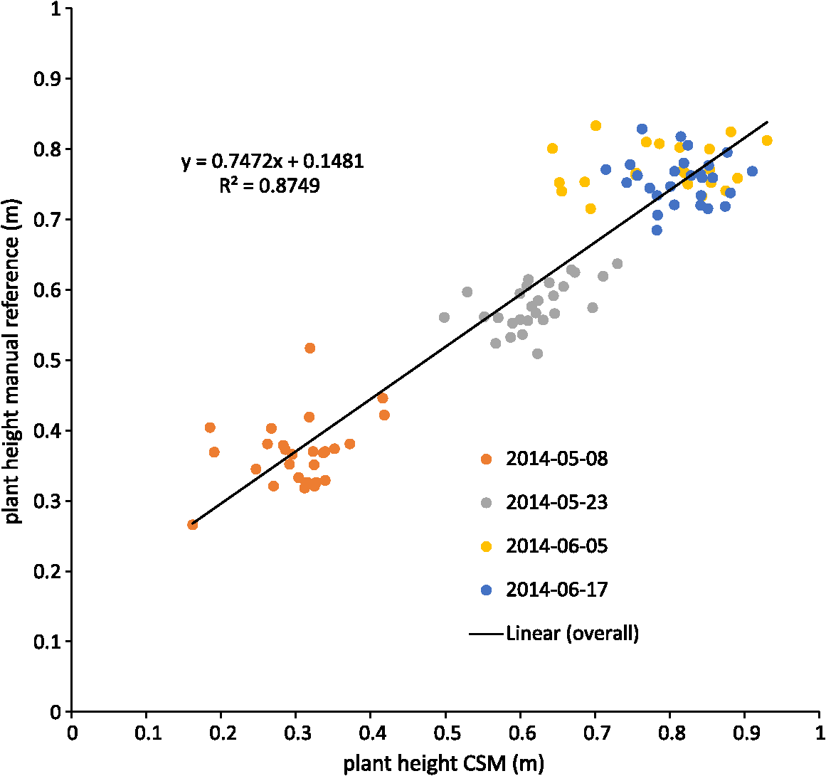

Figure 8 shows the mean plant height of the different cultivars over time: cultivar 4 had a faster growth in the early days after seeding. This can also be seen in the CSM for May 8 in Fig. 5. Cultivar 12, which showed the fastest growth in the CSM, was unfortunately not part of the set of cultivars selected for manual plant height measurements and, therefore, not included in the analysis here. Later in the growing season, cultivars 4 and 17 were higher, whereas cultivars 3 and 13 were smaller. The plant height values shown in this diagram are mean values of all mean values of all plots of the respective cultivar over all 3 CSMs/day. Generally, plant height increased until day 92 after seeding.

Fig. 8

Mean CSM-derived plant height per cultivar over time, trend line shows moving three-day average.

4.

Discussion

The high correlation values ($R^2>0.83$) (c.f., Table 2) and the similarity of the mean plant heights (c.f., Table 3) between CSM-derived plant heights and the manually measured plant heights showed the suitability of the presented system to monitor plant height on a field- to plot scale. The suitability of achieved point densities for different applications has been discussed in the literature^72,73 for LiDAR derived point clouds, and the general principles also apply for point clouds derived from stereo imagery. The linear regression of the CSM-derived plant heights with the manual plant height measurements showed the expected lower mean CSM plant heights per plot⁷⁴ compared to the manual plant height measurements in the early growing stages. The higher CSM plant heights in the late growing stage are not expected because we integrated the plant height measurements over the whole plot for the CSM derived measured. By doing so, lower parts of the plants were also included in the measurements, whereas the manual measurements considered only the maximum height of individual plants per plot.

Figure 8 shows that the semiautomated plant height monitoring over time was achieved successfully and that differences in plant height development over time between different cultivars could be observed, such as the fact that cultivar 1 grew faster earlier in the growing period compared to the other five cultivars. The slight downward trend at the end of the observation period can be explained by the fact that with ripening, the barley ears sank and thus height decreased. Small day to day variations in plant height could be explained by several factors: variations could be explained by the accuracy of the presented approach, representing noise in the measurement. Another possible explanation is that plant height could be affected by water availability; after precipitation events, plants can straighten up. A third possibility is wind; during windy conditions, the plants do not reach as high as in windless conditions.

Visual inspection of the generated CSMs also show different heights among the different cultivars: cultivar 12 showed faster growth in the first three CMSs shown in Fig. 5 compared to the other cultivars, but later experienced lodging, explaining the within-plot variations shown in the June 17 CSM.

For verification purposes, we compared our semiautomatically generated plant heights per plot with CSM-derived plant heights generated from UAV imagery, which have been shown to be reliable.^2,3 For this verification, we used the automatically generated CSMs with the highest number of plots with a point density $>100\text{points}/{\mathrm{m}}^2$ within 1 day of the UAV-based image acquisition. Figure 9 shows the linear regression between the derived mean plant heights per plot. As expected, a high coefficient of determination ($R^2=0.90$) was reached. Willmott’s index of model determination $d_r$ reached 0.94 while the RMSE was 0.13 m. The UAV-derived heights are generally lower than the plant heights derived from the 3-D monitoring system introduced in this study. A likely cause for this effect is the oblique image acquisition angle. Due to this angle, smaller plants could be obstructed in the oblique imagery because they were hidden by higher plants closer to the camera. In addition to this, the nadir viewing geometry of the UAV imagery results in more ground points being included in the generated dense point clouds. As the vegetation period continued and the crop canopy closed, less ground points were visible, and thus the difference decreased over time. Other studies^74,75 investigating oblique TLS measurements also suggest that plant heights should be higher in oblique viewing geometries when compared to measurements derived from angles closer to nadir.

Fig. 9

Regression of mean CSM-derived plant height and UAV-derived plant heights, UAV images acquired on May 06, May 20, June 06, and June 12.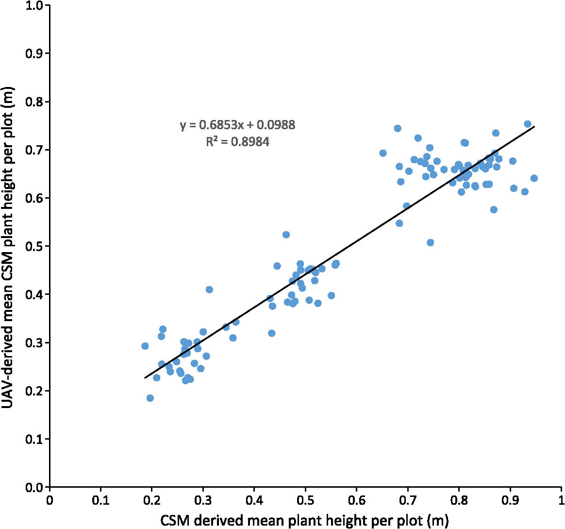

It is not clear why the automated GCP detection failed for at least one GCP marker in all image pairs. In some cases, in which weather conditions were sunny, the black and white GCP markers were overexposed, making it impossible for the black-and-white pattern to be automatically detected. However, even for images in which the GCP markers were not overexposed, the GCPs farther from the cameras were not detected, although their size in image space was sufficient (ca. $30\times 30\text{pixels}$). One possible explanation is that over time and depending on weather, the GCP markers became partially covered with dirt due to being placed directly on the bare-ground footpaths between the plots.

Figure 10 shows the achieved point densities: the point density decreases from $>5000/{\mathrm{m}}^2$ (spatial resolution $<1.5\mathrm{cm}$), in the areas closest to the cameras, to between 2500 and 500, in the front third of the field (allowing a spatial resolution of $<2\mathrm{cm}$), to between 2500 and 400 points in the rest of the field (allowing a spatial resolution of 5 cm). The focus area of key interest is contained in this area. Only for the parts farthest from the cameras, with a point density of at least 100, a spatial resolution of 10 cm is the best possible resolution. As expected, the drop-off in achieved point density with increasing camera distance corresponds roughly to the maximum achievable theoretical accuracy described in Sec. 2.2.7. The extent of the field that was covered by the generated point clouds, and therefore, the generated CSMs, changes between dates, c.f., Fig. 5. The areas that are not covered by all the generated point clouds lie at the far-end field, where the distance to the cameras is highest and the intersection angle is lowest. The depth map calculation algorithm apparently has problems calculating matching feature points at larger distances and lower intersection angles, and this varies from date to date probably due to different external imaging conditions such as wind and lighting. The key area of interest, the plots for which the monitoring design was developed (front third to the center of the field), is not affected by this problem.

Fig. 10

Point $\text{density}/{\mathrm{m}}^2$ for May 08, noon.

To be able to achieve a fully automatic monitoring in the future, two approaches need to be evaluated: first, a system in which the camera positions are completely fixed, e.g., by mounting the cameras on a fixed pole without hydraulics, should be examined. In the monitoring station setup presented in this study, where the cameras are mounted on a hydraulic lifting hoist, the camera positions slightly changed due to thermal expansion and compression of the hydraulic fluid. If the camera positions were truly fixed, full automation could be achieved by manually locating the GCP markers in one pair of acquired images just after the monitoring station has been setup and then using these manually determined pixel coordinates for all other image pairs acquired after that. Full automation would be possible because the GCP position in the images would stay fixed as long as both cameras and GCPs are stationary.

Second, a custom algorithm for detecting the GCPs could be implemented that takes into account additional information that is known due to the number of GCPs and the relative position of the GCPs and the cameras to each other (six GCPs per image, three GCPs in the top half of the image, two GCPs in each third of the image). This custom algorithm would, however, need to be individually adjusted each time a new field is observed. Another possible improvement to prevent overexposure in sunny conditions would be to change the GCPs to not be black and white, but black and gray instead. To prevent the GCP markers from becoming covered with dirt, they could be mounted slightly elevated. This would also make it possible to place them angled toward the cameras and make it possible to skip the distortion step mentioned earlier.

Another point worth discussing is the validity and direct comparability of mean plant heights derived from manual measurements with the CSM-derived plant heights. For the CSM-derived mean plot heights, the points in the dense point cloud do not represent the height of individual plants, but the top of the canopy instead. In contrast, with the manual measurement approach used here, 10 plants in each plot have their height measured individually. Alternative approaches for the manual plant height measurements that result in a better comparability with CSM-derived heights should be investigated in the future.

5.

Conclusions and Outlook

The overall aim of this study was to establish a low-cost semiautomated system for crop surface monitoring using oblique red, green, blue (RGB) imagery from consumer-grade smart cameras. 3-D plant height information was successfully derived from these images using SfMand MVS software. Improvements of the system could be implemented by increasing the reliability of the power supply to provide permanent interruption-free monitoring. Compared to other cost-intensive systems for 3-D plant monitoring, such as terrestrial or airborne laser scanning, this study presents a low-cost alternative. This low-cost goal has been mainly achieved by using consumer-grade cameras. While some of the software packages used in this study (Agisoft Photoscan and ArcGIS) are commercial and not free, the GIS processing performed in ArcGIS can also be performed with a free GIS system such as QGIS, as mentioned in Sec. 2.3. Overall, the cost of this system is significantly lower than a permanent installation of a TLS system, because the cheapest TLS systems that are able to cover a similar area cost tens of thousands of US dollars. The cameras used in this study cost just hundreds of dollars, with total costs $<4000$ dollars.

Summarizing, this study presents a semiautomated system for 3-D plant monitoring suitable for day-to-day monitoring with potential use in phenotyping. Future work should focus on several areas: (i) The investigation of whether it is possible to adapt this automated system to UAV-based image processing, therefore allowing the monitoring of a larger area by including more images acquired from a single UAV-based camera. To be able to examine how varying camera height and distance between cameras affect the quality of the results, future studies should include variation of these parameters. (ii) The feasibility of this system for biomass prediction based on the CSM-derived plant heights, analogous to the work of Bendig et al.⁵ and Tilly et al.⁴ (iii) The option of integrating other consumer-grade cameras with superior optics and larger sensors into this system, such as the Sony ICLE-QX1 mirrorless camera that features an APS-C-size sensor and interchangeable optics. (iv) The possibility of achieving a more even distribution of point density by using multiple stations positioned around one field and merging the point clouds produced by these multiple stations. By doing so, the whole field could be covered with a spatial resolution of $<2\mathrm{cm}$, thus achieving uniform data quality which would be more suitable for phenotyping applications.