Remote sensing of atmospheric water vapor from synthetic aperture radar interferometry: case studies in Shanghai, China

Liang Chang; Min Liu; Lixin Guo; Xiufeng He; Guoping Gao

doi:10.1117/1.JRS.10.046032

30 December 2016 Remote sensing of atmospheric water vapor from synthetic aperture radar interferometry: case studies in Shanghai, China

Liang Chang, Min Liu, Lixin Guo, Xiufeng He, Guoping Gao

Author Affiliations +

Journal of Applied Remote Sensing, Vol. 10, Issue 4, 046032 (December 2016). https://doi.org/10.1117/1.JRS.10.046032

Abstract

The estimation of atmospheric water vapor with high resolution is important for operational weather forecasting, climate monitoring, atmospheric research, and numerous other applications. The 40 m×40 m and 30 m×30 m differential precipitable water vapor (ΔPWV) maps are generated with C- and L-band synthetic aperture radar interferometry (InSAR) images over Shanghai, China, respectively. The ΔPWV maps are accessed via comparisons with the spatiotemporally synchronized PWV measurements from the European Centre for Medium-Range Weather Forecasts Interim reanalysis at the finest resolution and global positioning system observations, respectively. Results reveal that the ΔPWV maps can be estimated from both C- and L-band InSAR images with an accuracy of better than 2.0 mm, which, therefore, demonstrates the ability of InSAR observations at both C- and L-band to detect the water vapor distribution with high spatial resolution.

1. Introduction

Atmospheric water vapor is one of the most important and most abundant greenhouse gases in the Earth’s atmosphere, keeping the temperature of the Earth surface above the freezing level, as well as playing an important role in many atmospheric processes over a wide range of temporal and spatial scales. The phase variability of water vapor in time and space affects the distribution of clouds and rainfall, the structure of atmospheric storm systems, the vertical stability of the atmosphere, the evolution of the weather, and the energy balance of the global climate system.¹^,² The concept of precipitable water vapor (PWV), which is also referred to as total column or integrated water vapor, is the total water vapor contained in an air column from the Earth’s surface to the top of the atmosphere, and it is a good indicator of the water vapor variability in the lower troposphere and related processes.³ Therefore, more accurate precipitation and severe weather forecasts, together with a better understanding of climate change could be achieved via improved monitoring of atmospheric water vapor.

Radiosonde is one of the most common techniques to monitor global atmospheric water vapor. However, the radiosonde observations are available only twice a day at most sites, and they are limited due to the high operational costs, as well as the poor coverage over oceans and in the Southern Hemisphere.⁴ Since the early 1990s, estimation of PWV using ground-based global positioning system (GPS) observations has been well investigated.²^,⁵^–¹¹ GPS has become increasingly an operational tool to monitor the PWV due to its advantages including continuous measurements in all weather conditions, high accuracy, long-term stability, and low cost. Unfortunately, high spatial resolution of the water vapor distribution is still difficult to obtain in areas of sparse GPS sites.

Space-borne based monitoring is an effective way to estimate water vapor distribution with high resolution. A number of launched space-borne sensors can be used to extract the PWV measurements, such as the moderate resolution imaging spectroradiometer,¹² the medium resolution imaging spectrometer,¹³ the atmospheric infrared sounder,¹⁴ the infrared atmospheric sounding interferometer,¹⁵ the microwave radiometers,¹⁶ the Tropical Rainfall Measuring Mission’s Microwave Imager,¹⁷ the global precipitation measurement microwave imager,¹⁷ etc. However, these sensors can provide the PWV measurements only with a resolution of several kilometers, which may remain insufficient for the small scale weather forecasts. The synthetic aperture radar interferometry (InSAR) technique is a potential way to measure the PWV distribution with a resolution up to several meters.¹⁸ Considering the SAR signal delay caused by atmospheric water vapor is one of the major sources of noise for the InSAR technique,¹⁹ accurate surface deformation can be obtained after mitigating InSAR atmospheric distortions effectively.²⁰^–²⁴ In this study, we aim to estimate and evaluate the PWV distributions with C- and L-band InSAR observations when the surface deformation can be neglected during the time between the SAR image pairs acquisition. Cheng et al.²⁵ made a reliable comparison of atmospheric delay between GPS zenith tropospheric delay and SAR atmospheric phase screen in both differential and pseudoabsolute modes. Mateus et al.²⁶^–²⁸ emphasized that the PWV spatial distribution with a sampling period of a few days can be obtained by processing time series of InSAR images from different tracks of the same satellite and/or different space-borne missions. Efforts to construct accurate atmospheric water vapor distributions were also made by integrating persistent scatterer InSAR and global navigation satellite systems observations.²⁹^,³⁰ Recently, a few papers have also been published to measure the three-dimensional (3-D) state of the atmospheric water vapor by bridging InSAR and GPS tomography.³¹^–³³ However, most published works were exhibited using the C-band Environmental Satellite (ENVISAT) advanced SAR (ASAR) image pairs only, whereas the abilities of InSAR images at other bands in estimating the PWV measurements may need to be further inspected. In this study, both the C- and L-band InSAR observations are used to estimate the atmospheric water vapor maps over Shanghai, China. Moreover, the derived water vapor distributions are accessed via comparison with the spatiotemporally synchronized European Centre for Medium-Range Weather Forecasts (ECMWF) Interim reanalysis (ERA-Interim) data and GPS observations.

The rest of this paper is structured as follows. Section 2 introduces the principles of PWV estimation with GPS and InSAR observations. Section 3 describes the datasets used in this study and the InSAR data processing method. In Sec. 4, case studies of C- and L-band InSAR water vapor estimation in Shanghai, China, and their assessments are presented. Finally, some conclusions are addressed in Sec. 5.

2. Microwave Phase Delay in GPS and InSAR Observations

2.1.

GPS PWV Estimation

When traveling from the GPS satellites to the ground-based GPS receivers, the radio (microwave) signals are delayed by the ionosphere and neutral atmosphere. The ionospheric delay is frequency-dependent and can be removed by 99% with the data from dual-frequency GPS receivers.³⁴ The total tropospheric delay can then be expressed as²^,⁵

Eq. (1)

Δ L = ZHD \cdot m_{h} (ϵ) + ZWD \cdot m_{w} (ϵ),

where ZHD is the zenith hydrostatic delay, ZWD is the zenith wet delay,

ϵ

is the satellite elevation angle,

m_{h} (ϵ)

is the hydrostatic mapping function, and

m_{w} (ϵ)

is the wet mapping function.

The total tropospheric delay in the vertical direction (i.e., ZTD) is the sum of ZHD and ZWD,³⁵ and the former can be estimated by³⁶

Eq. (2)

ZHD = (2.2779 \pm 0.0024) P_{s} / [1 - 0.00266 \cos (2 φ) - 0.00028 h],

where

P_{s}

is the pressure (millibars) at the Earth’s surface,

φ

is the latitude, and

h

is the height above the ellipsoid (kilometres). Considering ZTD can be estimated from GPS observations [e.g., with the GPS analysis at Massachusetts Institute of Technology (GAMIT) software], ZWD can then be extracted by subtracting ZHD from ZTD. Moreover, PWV can be estimated from ZWD via a dimensionless parameter

Π

Eq. (3)

PWV = Π \times ZWD,

Eq. (4)

1 / Π = 10^{- 6} (K_{2}^{'} + K_{3} / T_{m}) R_{v},

where

T_{m}

is the water-vapor-weighted mean temperature

T_{m}

,

R_{v}

is the specific gas constant for water vapor, and

K_{3}

and

K_{2}^{'}

are the physical constants and given by Bevis et al.²

2.2.

Atmospheric Delay Feature in InSAR Interferograms

The atmospheric delay in SAR observations consists of bending and propagation delay, whereas the former can be neglected for zenith angles $< 87 \deg$ .³⁷ Therefore, the total zenith atmospheric delay can be expressed as³⁸

Eq. (5)

Δ L = ZHD + ZWD + Δ d_{ion} + Δ d_{liq},

where

Δ d_{ion}

is the zenith ionospheric delay and

Δ d_{liq}

is the zenith liquid delay caused by liquid water in the air. Liquid water delay is neglected due to its amplitude being

< 1 mm

under usual atmospheric circumstances,³⁸ whereas the ionosphere delay is regarded as minimal in low latitude regions.

For repeat-pass InSAR, the interferometric phase is the phase difference between the master and slave images, and the phase delay in InSAR observations can be expressed as

Eq. (6)

φ_{atm} = \frac{4 π}{λ} \cdot [\frac{Δ ZHD}{m_{h} (θ)} + \frac{Δ ZWD}{m_{w} (θ)}],

where

λ

is the wave length,

θ

is the incidence angle, and

Δ ZHD

and

Δ ZWD

are the difference of ZHD and ZWD between the master and slave images, respectively. Considering the minimal spatial variation and temporal stability of ZHD (1-mm accuracy of prediction),³⁸ the hydrostatic part is neglected in this study.

When the interferometric pairs used for atmospheric studies are acquired with a short-time interval, the deformation contribution during intervals between the SAR images overpass time can be considered as negligible, and the coherent interferometric phase can then be assumed due to the atmospheric propagation delay only and not related to surface deformation.²⁶ As such, the coherent interferometric phase can finally be converted to the PWV distribution variation by Eqs. (3) and (4).

3. Data Processing and Dataset

3.1.

Region of Interest and Datasets

In this study, four ENVISAT ASAR and three Advanced Land Observing Satellite (ALOS) Phased Array type L-band SAR (PALSAR) images are used to generate the InSAR interferograms (Ifms), respectively. As described in Table 1, the ASAR images were acquired in ascending orbit on June 30, 2008, August 4, 2008, September 8, 2008, and November 17, 2008, respectively, and the PALSAR images were acquired on August 27, 2008, October 12, 2008, and November 27, 2008, respectively. As a result, three C-band and two L-band Ifms are generated. It is also shown in Table 1 that the timespans between the master and slave images of the generated Ifms are all $< 70$ days. Considering the maximum subsidence rate of Shanghai in 2008 was $\sim 15 mm / year$ ,³⁹ the amount of deformation corresponding to a 70-day interval is, therefore, $< 2.9 mm$ when assuming that the deformation is temporally linear. Therefore, the deformation contribution to the interferometric phases can be considered as negligible in this study, since it can cause a phase shift of about only 0.05 cycles.²⁰

Table 1

Details of Ifms used in this study (track for ASAR and path for PALSAR, respectively).

Platform	Ifm	Master	Slave	Track/path	Time span (days)	B⊥ (m)a
C-band ENVISAT	Ifm1	June 30,2008	August 04, 2008	497	35	140 to 144
	Ifm2	August 04, 2008	September 08, 2008	497	35	312 to 327
	Ifm3	September 08, 2008	November 17, 2008	497	70	−160 to −137
L-band ALOS	Ifm4	August 27, 2008	October 12, 2008	441	46	1045 to 1066
L-band ALOS	Ifm5	October 12, 2008	November 27, 2008	441	46	−253 to −241

^aPerpendicular baseline at center of swath.

Figure 1 shows the location of the region of interest (ROI) and the coverages of the ASAR and PALSAR images, respectively. In this study, a total of 11 GPS stations are located inside the ROI. The GPS data are used to estimate the PWV measurements, and further assess the accuracy of InSAR derived PWV distributions. In order to obtain accurate GPS baseline solutions and ZWD measurements, we process the GPS data in double-difference phase baseline mode with the GAMIT 10.60 software and extract the ZWD series for 30-min intervals.

Fig. 1

Locations of the SAR images used in this study and the GPS stations around the ROI with 3-arc sec SRTM shaded relief. Purple and brown boxes represent the ASAR and PALSAR interferometric pairs, respectively, black solid triangles show GPS stations, and red crosses denote the locations of ERA-Interim grids.

ERA-Interim is a third generation of comprehensive global reanalysis, which uses a much improved atmospheric model and assimilation system from those used in ERA-40.⁴⁰ ERA-Interim represents a major undertaking by ECMWF with several of the inaccuracies exhibited by ERA-40 being eliminated or significantly reduced. In this study, total column water vapor from ERA-Interim at the finest resolution (i.e., $0.125 \deg \times 0.125 \deg$ ) every 6 h (i.e., 00, 06, 12, and 18 h) is adopted to compare with the InSAR derived PWV distributions. It should be noted that the spline interpolation is used for PWV time-series from ERA-Interim data to get the PWV measurements at SAR overpass time.

3.2.

InSAR Data Processing

In this paper, the SAR images are processed with GAMMA Remote Sensing software by the two-pass differential InSAR approach. Precise DORIS orbit data provided by the European Space Agency (ESA) are used to reduce baseline errors, assist image coregistration, and remove flat earth phase of ASAR interferometric pairs. The digital elevation model (DEM) with nominal 90-m sample spacing provided by the National Aeronautics and Space Administration (NASA) Shuttle Radar Topography Mission (SRTM) is employed to simulate the height map in the radar coordinates system and to mitigate the topographic phase in the Ifms. To suppress the noise in the Ifms, the C-band ASAR (L-band PALSAR) interferometric pairs are processed by a multilooking operation with 10 pixels in azimuth and 2 pixels (4 pixels) in range directions to get a final resolution of about $40 m \times 40 m$ ( $30 m \times 30 m$ ).

The coherence values of the C- and L-band Ifms are shown in Fig. 2. A mean coherence of 0.90, 0.86, and 0.91 is observed in C-band Ifm1, Ifm2, and Ifm3, respectively. The slightly low coherence in Ifm2 [Fig. 2(b)] may lie in the longer perpendicular baseline of Ifm2 compared with Ifm1 and Ifm3 (Table 1). In addition, a mean coherence of 0.96 is also detected in L-band Ifm4 and Ifm5. It should be mentioned that despite the perpendicular baseline of Ifm4 being longer than that of Ifm1, the coherence in the former is higher than the latter. The significant coherence gain in L-band Ifms may result from the longer wavelength of ALOS PALSAR and therefore the better penetration than ENVISAT ASAR. Moreover, the coherence in each Ifm is in general higher over the city of Shanghai and part of Pudong, Jiading, Minghang, Fengxian, and Songjiang districts than Changxing, Hengsha, and Chongming islands.

Fig. 2

Coherence maps from C- (a)–(c) and L-band (d) and (e) InSAR images with SRTM shaded relief acquired on: (a) June 30 and August 4, 2008; (b) August 4 and September 8, 2008; (c) September 8 and November 17, 2008; (d) August 27 and October 12, 2008; and (e) October 12 and November 27, 2008, respectively.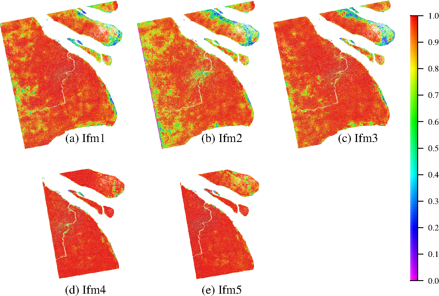

The Ifms are then smoothed by adaptive filtering and unwrapped by the branch-cut method with the coherence threshold set to be 0.5. The baselines are refined next using the unwrapped phase and the independent DEM, which can help to generate more reasonable values for areas with low coherence. Moreover, a two-dimensional quadratic model phase function from the differential Ifm is also estimated to mitigate possible orbital errors. At last, the unwrapped Ifms are mapped into the line of sight (LOS) direction in the Universal Transverse Mercator coordinate system. Figure 3 shows the unwrapped interferometric phases of the C- and L-band Ifms. It is clear that there are no apparent systematic phase trends in Fig. 3. Considering the “bridges” construction may introduce extra errors during the phase unwrapping processes, as well as prevent objective assessment of InSAR derived PWV distributions, we have not constructed the “bridges” between the center area and the islands. As a result, the unwrapped interferometric phases over the areas of Changxing Island, Hengsha Island, Chongming Island, and Qidong City are masked.

Fig. 3

Same as in Fig. 2, but for unwrapped phases.

4. Assessment of PWV Measurements from InSAR Observations

4.1.

Comparison of PWV Maps Between InSAR and ERA-Interim Data

As analyzed in Sec. 2, the unwrapped interferometric phases in the radar LOS direction can be regarded as the slant total wet delay without considering the hydrostatic delay component. The LOS wet delay maps are then converted into the zenith direction with the simplest mapping function $1 / \cos θ$ , where $θ$ is the incidence angle of each SAR image pixel. The converted ZWD is further used to extract the differential PWV ( $Δ PWV$ ; master minus slave) distributions via the dimensionless quality in Eq. (3). Given that the ERA-Interim data at the finest resolution are still far sparser than InSAR Ifms, the $Δ PWV$ measurements from InSAR images are compared with ERA-Interim data at the locations of ERA-Interim grids only (i.e., on $0.125 \deg \times 0.125 \deg$ grid).

4.1.1.

C-band ENVISAT ASAR

Figure 4 shows the comparison of $Δ PWV$ distributions from C-band InSAR Ifms and spatiotemporally synchronized ERA-Interim data, together with the spatial distributions and histograms of $Δ PWV$ differences. As we can see in Fig. 4(a) the negative $Δ PWV$ measurements are observed at the bottom left and top right of the Ifm1, with a severest negative signal of about $- 4.7 mm$ . In addition, positive signals are mainly found in the center of Ifm1 with the maximum amplitude of about 2.3 mm. The variation of $Δ PWV$ measurements in Ifm1 in terms of standard deviation (STD) is about 1.3 mm, together with that STD in spatiotemporally synchronized ERA-Interim grids [Fig. 4(b)] is 1.9 mm. As a result, an overall STD of 1.9 mm for the $Δ PWV$ differences (InSAR minus ERA-Interim) between Figs. 4(a) and 4(b) is detected in Fig. 4(c). Moreover, it can be detected from the histogram of Ifm1 [Fig. 4(d)] that the $Δ PWV$ differences generally range from $- 2$ to 2 mm with an overall root mean square (RMS) of about 1.9 mm.

Fig. 4

$Δ PWV$ distributions from C-band ENVISAT ASAR Ifms [(a), (e), (i)] and spatiotemporally synchronized ERA-Interim data [(b), (f), (j)], and the spatial distributions [(c), (g), (k)] and histograms [(d), (h),(l)] of their $Δ PWV$ differences. The top, middle, and bottom rows denote the results for Ifm1, Ifm2, and Ifm3, respectively.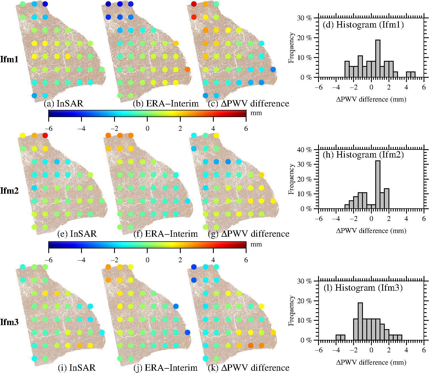

The C-band InSAR derived $Δ PWV$ distribution in Ifm2 [Fig. 4(e)] is surrounded by positive signals except that mild negative signals are found in the middle-north of the study area. In contrast, the $Δ PWV$ map estimated from ERA-Interim data [Fig. 4(f)] exhibits obvious gradient from northwest to southeast. The $Δ PWV$ variation in Ifm2 and spatiotemporally synchronized ERA-Interim data in terms of STD are about 1.3 and 1.2 mm, respectively, as well as the overall STD of their $Δ PWV$ differences is about 1.3 mm. In Fig. 4(h), inspiring results are also shown since their $Δ PWV$ differences occur more frequently from $- 1$ to 1 mm with an RMS of about 1.3 mm. The $Δ PWV$ variation in Ifm3 [Fig. 4(i)] and spatiotemporally synchronized ERA-Interim data [Fig. 4(j)] in terms of STD are about 1.0 and 1.3 mm, respectively, together with the overall STD of their $Δ PWV$ differences is about 1.6 mm [Fig. 4(k)]. Furthermore, the frequency histogram of $Δ PWV$ differences of Ifm3 [Fig. 4(l)] again demonstrates that the C-band InSAR derived $Δ PWV$ can be estimated with an accuracy of $< 2.0 mm$ when compared with spatiotemporally synchronized ERA-Interim data.

The probable cause for the $Δ PWV$ differences between InSAR and spatiotemporally synchronized ERA-Interim data may result from uncertainties existing in the latter, as well as the errors introduced by interpolating the ERA-Interim PWV time series. Moreover, the uncertainties in InSAR data processing (e.g., phase errors induced by the SRTM height uncertainties, baseline errors, etc.) and temporal variations of ZHD between the acquire time of the master and slave images may also contribute to the discrepancies of $Δ PWV$ differences.

4.1.2.

L-band ALOS PALSAR

Figure 5 shows the comparisons of $Δ PWV$ distributions from L-band PALSAR Ifms and spatiotemporally synchronized ERA-Interim data, together with the spatial distributions and histograms of $Δ PWV$ differences. Unlike only mild $Δ PWV$ variation (from $- 0.4$ to 0.6 mm) is observed in Ifm4 [Fig. 5(a)], obvious $Δ PWV$ variation (from $- 5.3$ to 3.7 mm) is found from spatiotemporally synchronized ERA-Interim data [Fig. 5(b)]. The $Δ PWV$ variation in Figs. 5(a) and 5(b) in terms of STD is about 0.3 and 2.2 mm, respectively, together with the overall STD of their $Δ PWV$ differences is about 2.3 mm [Fig. 5(c)]. As we can see in Fig. 5(d), the histogram of $Δ PWV$ differences of Ifm4 suggests obvious negative $Δ PWV$ signals around $- 2 mm$ . The most probable reason for the large $Δ PWV$ differences in Ifm4 may be the perpendicular baseline length of exceeding 1000 m, which results in the sensitivity of the Ifm to the DEM errors and therefore introduces extra residual phases.

Fig. 5

Same as in Fig. 4, but for L-band ALOS PALSAR Ifms. The top and bottom rows denote the results for Ifm4 and Ifm5, respectively.

The $Δ PWV$ distribution in Ifm5 [Fig. 5(e)] is in good agreement with that from spatiotemporally synchronized ERA-Interim data [Fig. 5(f)]. The $Δ PWV$ variation in Figs. 5(e) and 5(f) in terms of STD is about 0.3 and 0.7 mm, respectively, as well as the overall STD of their $Δ PWV$ differences is about 0.7 mm [Fig. 5(g)]. Furthermore, it can be observed from Fig. 5(g) that their $Δ PWV$ differences are all within $\pm 1.5 mm$ . Therefore, the L-band PALSAR InSAR images with proper perpendicular baseline length can also help to estimate the moisture distributions effectively.

4.2.

Validation of InSAR Derived ΔPWV Measurements with GPS Observations

GPS is able to estimate the PWV measurements with high temporal resolution and high precision, which makes it an ideal tool to validate the $Δ PWV$ distributions from InSAR images. In addition, the water vapor sensed by GPS observations is typically estimated by sampling throughout a conical section of the atmosphere above the GPS receiver. In this study, the GPS satellites cut-off elevation angle was set to 15 deg during the GPS data processing with the GAMIT 10.60 software. Therefore, the InSAR estimates are obtained by averaging all pixels located at a distance $< 5.23 km$ from the GPS station during the comparisons of $Δ PWV$ from InSAR and GPS data.¹⁹

4.2.1.

C-band ENVISAT ASAR

Figure 6 shows each $Δ PWV$ measurement from C-band ASAR Ifms and spatiotemporally synchronized GPS observations, as well as the histograms of their $Δ PWV$ differences. As can be seen in Fig. 6(a) the $Δ PWV$ measurements from ASAR unwrapped phases and GPS data show similar variation at all available GPS sites, except that the $Δ PWV$ differences are larger than 2 mm at SHBS, SHJS, and SHNH. As a result, an overall STD of 1.9 mm is obtained from the $Δ PWV$ differences between Ifm1 and spatiotemporally synchronized GPS data. In addition, the histogram of Ifm1 in Fig. 6(b) shows that their $Δ PWV$ differences are within $\pm 3 mm$ , with a mean of $- 0.8 mm$ at all GPS sites.

Fig. 6

Comparisons of $Δ PWV$ measurements from C-band InSAR Ifms and spatiotemporally synchronized GPS observations, together with the histograms of their $Δ PWV$ differences. Note that the top, middle, and bottom rows denote the results for (a) and (b) Ifm1, (c) and (d) Ifm2, and (e) and (f) Ifm3, respectively. Red solid squares and green solid triangles are the $Δ PWV$ measurements from InSAR Ifms and spatiotemporally synchronized GPS data, respectively. Yellow solid bars denote their $Δ PWV$ differences (InSAR minus GPS).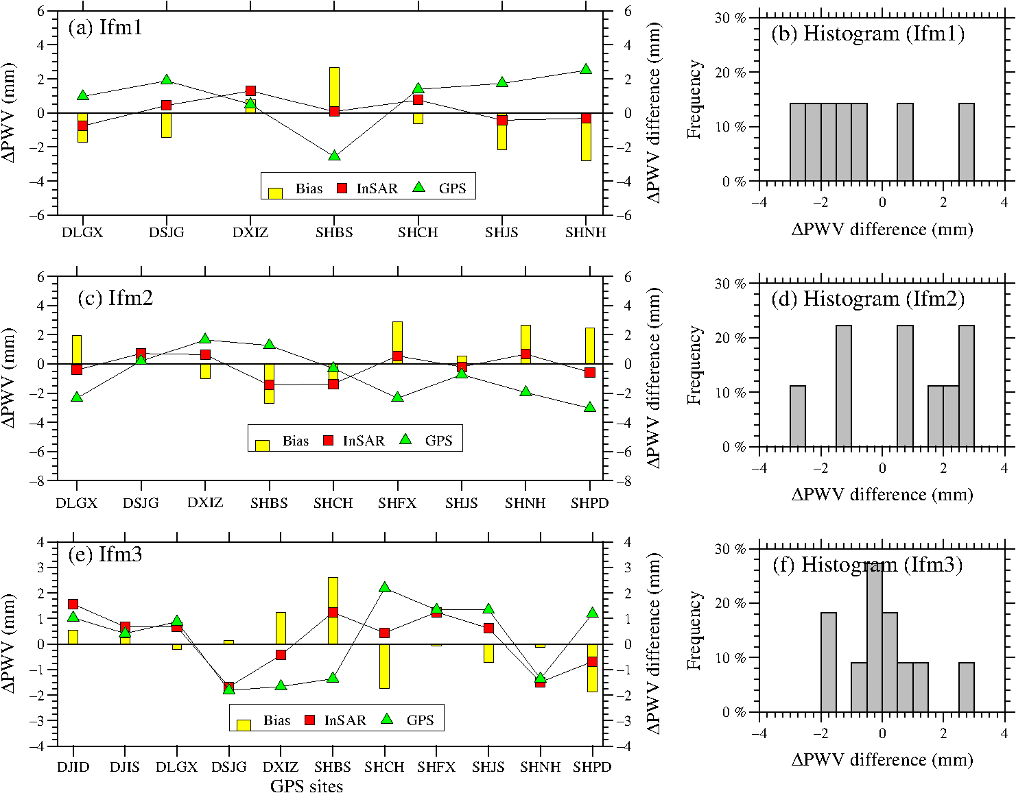

In Fig. 6(c), 9 of 11 GPS sites are available for $Δ PWV$ comparison from Ifm2 and spatiotemporally synchronized GPS data. The maximum $Δ PWV$ difference of 2.9 mm is found at SHFX, and the minimum $Δ PWV$ difference of 0.5 mm is found at DSJG. In addition, an STD of 2.0 mm and an overall mean of 0.7 mm are observed from their $Δ PWV$ differences [Fig. 6(d)]. As for the comparison in Ifm3 [Figs. 6(e)–6(f)], all $Δ PWV$ measurements at 11 GPS sites are estimated, and the $Δ PWV$ differences between Ifm3 and spatiotemporally synchronized GPS data are $< \pm 1 mm$ at 7 of 11 GPS sites. As a result, an STD of 1.3 mm is achieved during their $Δ PWV$ differences comparison, which shows better agreement than the comparisons of Ifm1 and Ifm2. Moreover, the histogram of their $Δ PWV$ differences [Fig. 6(f)] is close to normal distribution, with an overall mean of $Δ PWV$ differences close to zero.

4.2.2.

L-band ALOS PALSAR

Figure 7 shows the $Δ PWV$ measurements from L-band PALSAR Ifms and spatiotemporally synchronized GPS observations, as well as the histograms of their $Δ PWV$ differences. As we can see in Fig. 7(a), 6 of 7 GPS sites are available for the $Δ PWV$ comparison in Ifm4. The $Δ PWV$ differences between Ifm4 and spatiotemporally synchronized GPS data are within the range of $- 0.2$ to 0.9 mm for all the sites except for SHBS, which shows an RMS of 1.5 mm and an STD of 1.3 mm. Moreover, the histogram in Fig. 7(b) also illustrates that their $Δ PWV$ differences occur more frequently around zero with an overall mean of about $- 0.3 mm$ . In Figs. 7(c) and 7(d), all seven GPS sites are available for the comparison in Ifm5, and the $Δ PWV$ differences between Ifm5 and spatiotemporally synchronized GPS data range from $- 1.7$ to 1.9 mm for all the sites. Comparison of their $Δ PWV$ measurements in Ifm5 gives an overall mean of 0.5 mm and an RMS of 1.3 mm, which is a very good validation of this study.

Fig. 7

Same as in Fig. 6, but for L-band ALOS InSAR Ifms. The top and bottom rows denote the results for Ifm4 and Ifm5, respectively.

5. Conclusions

In this study, interferometric phases from C- and L-band InSAR images are incorporated to derive the atmospheric water vapor information with the high spatial resolution of $40 m \times 40 m$ and $30 m \times 30 m$ , respectively. We conduct analysis to extract the PWV measurements on three ASAR and two PALSAR image pairs over the city of Shanghai, China. Moreover, the estimated $Δ PWV$ distributions are accessed via comparisons with those results from spatiotemporally synchronized ERA-Interim grids and GPS observations.

Comparisons of $Δ PWV$ distributions from C-band ASAR Ifms and spatiotemporally synchronized ERA-Interim data show an overall STD of 1.9, 1.3, and 1.6 mm for Ifm1, Ifm2, and Ifm3, respectively, while those comparisons from L-band PALSAR Ifms and spatiotemporally synchronized ERA-Interim data give an overall STD of 2.3 and 0.7 mm for Ifm4 and Ifm5, respectively. The large discrepancies of $Δ PWV$ measurements from Ifm4 and spatiotemporally synchronized ERA-Interim data may result from the long perpendicular baseline of Ifm4. In addition, the comparisons of $Δ PWV$ maps from C-band ASAR Ifms and spatiotemporally synchronized GPS data give an STD of 1.9, 2.0, and 1.3 mm in Ifm1, Ifm2, and Ifm3, respectively. The STD of $Δ PWV$ differences from L-band PALSAR Ifms and spatiotemporally synchronized GPS data is 1.3 and 1.2 mm in Ifm4 and Ifm5, respectively. As such, it could be, therefore, concluded from this study that InSAR images can detect the $Δ PWV$ measurements with an RMS of better than 2.0 mm.

In addition, the water vapor information in plain areas is necessary for numerical forecasting procedures [e.g., those based on the 3-D variational data assimilation (3-DVAR) and four-dimensional variational data assimilation (4-DVAR) analysis], and PWV spatial distributions in high-altitude regions are also important for meteorologists to forecast precipitation and severe weather conditions. However, extractions of water vapor information from InSAR images in these areas are not conducted in this study, which would be an important issue in the future.

Acknowledgments

We would like to thank the extremely valuable suggestions from the editor (Prof. Ni-Bin Chang) and the two anonymous referees, who have put a considerable amount of time and effort into reviewing and improving this paper. We also thank the Alaska Satellite Facility (ASF) Distributed Active Archive Center (DAAC) for providing the ALOS data, and the ESA for providing the ENVISAT images. This work was funded by the Global Change Research Program of China (No. 2015CB953900), the National Natural Science Foundation of China (Nos. 41506211, 41276197, and 41475040), the Shanghai Oriental Scholar Program (No. 2012-58), the Shanghai Sailing Program (No. 14YF1410200), and the Innovation Program of Shanghai Municipal Education Commission (Nos. 14YZ118 and 14ZZ148).

References

1.

M. Chahine, “The hydrological cycle and its influence on climate,” Nature, 359 373 –380 (1992). http://dx.doi.org/10.1038/359373a0 Google Scholar

2.

M. Bevis et al., “GPS meteorology: mapping zenith wet delays onto precipitable water,” J. Appl. Meteorol., 33 379 –386 (1994). http://dx.doi.org/10.1175/1520-0450(1994)033<0379:GMMZWD>2.0.CO;2 Google Scholar

3.

O. Bock et al., “Multiscale analysis of precipitable water vapor over Africa from GPS data and ECMWF analyses,” Geophys. Res. Lett., 34 (9), L09705 (2007). http://dx.doi.org/10.1029/2006GL028039 Google Scholar

4.

Z. Li, J. P. Muller and P. Cross, “Comparison of precipitable water vapor derived from radiosonde, GPS, and moderate-resolution imaging spectroradiometer measurements,” J. Geophys. Res., 108 (D20), 4651 (2003). http://dx.doi.org/10.1029/2003JD003372 Google Scholar

5.

M. Bevis et al., “GPS meteorology: remote-sensing of atmospheric water vapor using the global positioning system,” J. Geophys. Res., 97 15787 –15801 (1992). http://dx.doi.org/10.1029/92JD01517 JGREA2 0148-0227 Google Scholar

6.

S. Businger et al., “The promise of GPS in atmospheric monitoring,” Bull. Am. Meteorol. Soc., 77 5 –18 (1996). http://dx.doi.org/10.1175/1520-0477(1996)077<0005:TPOGIA>2.0.CO;2 BAMIAT 0003-0007 Google Scholar

7.

J. Duan et al., “GPS meteorology: direct estimation of the absolute value of precipitable water,” J. Appl. Meteorol., 35 830 –838 (1996). http://dx.doi.org/10.1175/1520-0450(1996)035<0830:GMDEOT>2.0.CO;2 Google Scholar

8.

C. Rocken et al., “Sensing atmospheric water vapor with the global positioning system,” Geophys. Res. Lett., 20 2631 –2634 (1993). http://dx.doi.org/10.1029/93GL02935 GPRLAJ 0094-8276 Google Scholar

9.

C. Rocken et al., “Near real-time GPS sensing of atmospheric water vapor,” Geophys. Res. Lett., 24 3221 –3224 (1997). http://dx.doi.org/10.1029/97GL03312 GPRLAJ 0094-8276 Google Scholar

10.

P. Tregoning et al., “Accuracy of absolute precipitable water vapor estimates from GPS observations,” J. Geophys. Res., 103 28701 –28710 (1998). http://dx.doi.org/10.1029/98JD02516 JGREA2 0148-0227 Google Scholar

11.

L. Chang et al., “Regional precipitation forecast using GPS and NCEP,” Sci. Sin. Phys. Mech. Astron., 40 (5), 685 –692 (2010). http://dx.doi.org/10.1360/2010-40-5-685 Google Scholar

12.

L. Chang et al., “Calibration and evaluation of precipitable water vapor from MODIS infrared observations at night,” IEEE Trans. Geosci. Remote Sens., 53 (5), 2612 –2620 (2015). http://dx.doi.org/10.1109/TGRS.2014.2363089 Google Scholar

13.

Z. H. Li et al., “Assessment of the potential of MERIS near-infrared water vapour products to correct ASAR interferometric measurements,” Int. J. Remote Sens., 27 (2), 349 –365 (2006). http://dx.doi.org/10.1080/01431160500307342 Google Scholar

14.

S. Bedka et al., “An assessment of the absolute accuracy of the atmospheric infrared sounder v5 precipitable water vapor product at tropical, midlatitude, and arctic ground-truth sites: September 2002 through August 2008,” J. Geophys. Res. Atmos., 115 (D17), D17310 (2010). http://dx.doi.org/10.1029/2009JD013139 Google Scholar

15.

F. Aires et al., “Remote sensing from the infrared atmospheric sounding interferometer instrument-2. Simultaneous retrieval of temperature, water vapor, and ozone atmospheric profiles,” J. Geophys. Res. Atmos., 107 (D22), 4620 (2002). http://dx.doi.org/10.1029/2001JD001591 Google Scholar

16.

A. Somieski et al., “Tropospheric water vapor from solar spectrometry and comparison with Jason microwave radiometer measurements,” J. Geophys. Res. Atmos., 111 (D9), D09104 (2006). http://dx.doi.org/10.1029/2005JD005767 Google Scholar

17.

G. W. Petty and K. Li, “Improved passive microwave retrievals of rain rate over land and ocean. Part I: algorithm description,” J. Atmos. Oceanic Technol., 30 (11), 2493 –2508 (2013). http://dx.doi.org/10.1175/JTECH-D-12-00144.1 Google Scholar

18.

R. F. Hanssen, “High-resolution water vapor mapping from interferometric radar measurements,” Science, 283 (5410), 2020 –2020 (1999). http://dx.doi.org/10.1126/science.283.5406.1297 SCIEAS 0036-8075 Google Scholar

19.

R. Hanssen, Atmospheric Heterogeneities in ERS Tandem SAR Interferometry, Delft University Press, Delft, Netherlands (1998). Google Scholar

20.

L. Chang and X. F. He, “InSAR atmospheric distortions mitigation: GPS observations and NCEP FNL data,” J. Atmos. Sol. Terr. Phys., 73 (4), 464 –471 (2011). http://dx.doi.org/10.1016/j.jastp.2010.11.003 Google Scholar

21.

L. Chang, S. G. Jin and X. F. He, “Assessment of InSAR atmospheric correction using both MODIS near-infrared and infrared water vapor products,” IEEE Trans. Geosci. Remote Sens., 52 (9), 5726 –5735 (2014). http://dx.doi.org/10.1109/TGRS.2013.2292070 Google Scholar

22.

Z. H. Li et al., “MERIS atmospheric water vapor correction model for wide swath interferometric synthetic aperture radar,” IEEE Geosci. Remote Sens. Lett., 9 (2), 257 –261 (2012). http://dx.doi.org/10.1109/LGRS.2011.2166053 Google Scholar

23.

Z. W. Li et al., “Correcting atmospheric effects on InSAR with MERIS water vapour data and elevation-dependent interpolation model,” Geophys. J. Int., 189 (2), 898 –910 (2012). http://dx.doi.org/10.1111/gji.2012.189.issue-2 Google Scholar

24.

C. J. Xu et al., “InSAR tropospheric delay mitigation by GPS observations: a case study in Tokyo area,” J. Atmos. Sol.-Terr. Phys., 68 (6), 629 –638 (2006). http://dx.doi.org/10.1016/j.jastp.2005.11.010 Google Scholar

25.

S. L. Cheng et al., “Atmospheric delay analysis from GPS meteorology and InSAR APS,” J. Atmos. Sol.-Terr. Phys., 86 71 –82 (2012). http://dx.doi.org/10.1016/j.jastp.2012.06.005 Google Scholar

26.

P. Mateus, G. Nico and J. Catalao, “Can spaceborne SAR interferometry be used to study the temporal evolution of PWV?,” Atmos. Res., 119 70 –80 (2013). http://dx.doi.org/10.1016/j.atmosres.2011.10.002 Google Scholar

27.

P. Mateus, G. Nico and J. Catalao, “Mapping temporal evolution of water vapour in troposphere by interferometric SAR data,” Proc. SPIE, 7827 782712 (2010). http://dx.doi.org/10.1117/12.864727 Google Scholar

28.

P. Mateus, G. Nico and J. Catalao, “Maps of PWV Temporal Changes by SAR Interferometry: a study on the properties of atmosphere’s temperature profiles,” IEEE Geosci. Remote Sens. Lett., 11 (12), 2065 –2069 (2014). http://dx.doi.org/10.1109/LGRS.2014.2318993 Google Scholar

29.

F. Alshawaf et al., “Water vapor mapping by fusing InSAR and GNSS remote sensing data and atmospheric simulations,” Hydrol. Earth Syst. Sci., 19 (12), 4747 –4764 (2015). http://dx.doi.org/10.5194/hess-19-4747-2015 Google Scholar

30.

F. Alshawaf et al., “Constructing accurate maps of atmospheric water vapor by combining interferometric synthetic aperture radar and GNSS observations,” J. Geophys. Res. Atmos., 120 (4), 1391 –1403 (2015). http://dx.doi.org/10.1002/2014JD022419 Google Scholar

31.

M. Heublein et al., “Compressive sensing for neutrospheric water vapor tomography using GNSS and InSAR Observations,” in IEEE Int. Geoscience and Remote Sensing Symp. (IGARSS ‘15), 5268 –5271 (2015). http://dx.doi.org/10.1109/IGARSS.2015.7327023 Google Scholar

32.

P. Benevides et al., “Merging SAR interferometry and GPS tomography for high-resolution mapping of 3D tropospheric water vapour,” in IEEE Int. Geoscience and Remote Sensing Symp. (IGARSS ‘15), 3607 –3610 (2015). http://dx.doi.org/10.1109/IGARSS.2015.7326602 Google Scholar

33.

P. Benevides et al., “Bridging InSAR and GPS tomography: a new differential geometrical constraint,” IEEE Trans. Geosci. Remote Sens., 54 (2), 697 –702 (2016). http://dx.doi.org/10.1109/TGRS.2015.2463263 Google Scholar

34.

F. Brunner and M. Gu, “An improved model for the dual frequency ionospheric correction of GPS observations,” Manuscripta Geodetica, 16 (3), 205 –214 (1991). Google Scholar

35.

J. Saastamoinen, “Atmospheric correction for the troposphere and stratosphere in radio ranging of satellites,” The Use of Artificial Satellites for Geodesy, 15 (6), 245 –251 American Geophysical Union, Washington, DC (1972). Google Scholar

36.

G. Elgered et al., “Geodesy by radio interferometry: water vapor radiometry of estimation of the wet delay,” J. Geophys. Res., 96 6541 –6555 (1991). http://dx.doi.org/10.1029/90JB00834 JGREA2 0148-0227 Google Scholar

37.

B. R. Bean and E. J. Dutton, Radio Meteorology, Dover, New York (1968). Google Scholar

38.

R. F. Hanssen, Radar Interferometry: Data Interpretation and Error Analysis, Kluwer Academic, Dordrecht, Boston (2001). Google Scholar

39.

M.S. Liao et al., “Analyzing TerraSAR-X and COSMO-SkyMed high-resolution SAR data of urban areas,” in Proc. ISPRS Workshop High-Resolution Earth Imaging for Geospatial Information, (2009). Google Scholar

40.

D. P. Dee et al., “The ERA-Interim reanalysis: configuration and performance of the data assimilation system,” Q. J. R. Meteorolog. Soc., 137 (656), 553 –597 (2011). http://dx.doi.org/10.1002/qj.v137.656 Google Scholar

Biography

Liang Chang received his BEng degree in surveying and mapping engineering from Nanjing University of Technology, China, in 2006, and his PhD in geodesy and surveying engineering from Hohai University, China, in 2011. From July 2011 to May 2013, he was a postdoctoral fellow at Shanghai Astronomical Observatory (SHAO), Chinese Academy of Sciences (CAS), China. He is currently a lecturer at Shanghai Ocean University, China. His research interests include GNSS meteorology, InSAR, and satellite oceanography.

Min Liu received her BSc degree in information and computing science from Nanjing University of Information Science and Technology, Nanjing, China, in 2003, and her MSc degree in astrometry and celestial mechanics from SHAO, CAS, Shanghai, China, in 2006. She started a PhD in geodesy from Hong Kong Polytechnic University in 2011. She is currently a senior engineer of Shanghai Meteorological Bureau, Shanghai, China. Her research interests include GNSS meteorology and high-precision positioning.

Lixin Guo: Biography is not available.

Xiufeng He received her BEng and MS degrees in control and navigation from Nanjing University of Aeronautics and Astronautics, China, in 1986 and 1989 respectively, and her PhD in navigation and survey engineering from Hong Kong Polytechnics University in 1998. She was a postdoctoral fellow at Norwegian University of Science and Technology in 1998–1999 and a research fellow at Singapore Nanyang Technological University in 2000. She is currently a professor at Hohai University, China.

Guoping Gao received his BSc degree in meteorology from Ocean University of China (OUC), China, in 1994 and his PhD in marine science from the University of Massachusetts (UMASS), USA, in 2011. From July 1994 to March 2005, he was an engineer in ocean observation in the OUC, China. From March 2005 to September 2006, he has been a visiting scholar at UMASS, USA. He is currently a professor at Shanghai Ocean University, China.

CC BY: © The Authors. Published by SPIE under a Creative Commons Attribution 4.0 Unported License. Distribution or reproduction of this work in whole or in part requires full attribution of the original publication, including its DOI.

Citation Download Citation

Liang Chang, Min Liu, Lixin Guo, Xiufeng He, and Guoping Gao "Remote sensing of atmospheric water vapor from synthetic aperture radar interferometry: case studies in Shanghai, China," Journal of Applied Remote Sensing 10(4), 046032 (30 December 2016). https://doi.org/10.1117/1.JRS.10.046032

Received: 17 June 2016; Accepted: 5 December 2016; Published: 30 December 2016

Access the abstract

JOURNAL ARTICLE
13 PAGES

DOWNLOAD PAPER SAVE TO MY LIBRARY

GET CITATION

CITATIONS

Cited by 4 scholarly publications.

Explore citations on Lens.org

KEYWORDS

Interferometric synthetic aperture radar

Global Positioning System

Interferometry

Synthetic aperture radar

L band

Atmospheric sensing

Remote sensing

1.

Introduction

2.

Microwave Phase Delay in GPS and InSAR Observations

2.1.

GPS PWV Estimation

Eq. (1)

Eq. (2)

Eq. (3)

Eq. (4)

2.2.

Atmospheric Delay Feature in InSAR Interferograms

Eq. (5)

Eq. (6)

3.

Data Processing and Dataset

3.1.

Region of Interest and Datasets

Table 1

Fig. 1

3.2.

InSAR Data Processing

Fig. 2

Fig. 3

4.

Assessment of PWV Measurements from InSAR Observations

4.1.

Comparison of PWV Maps Between InSAR and ERA-Interim Data

4.1.1.

C-band ENVISAT ASAR

Fig. 4

4.1.2.

L-band ALOS PALSAR

Fig. 5

4.2.

Validation of InSAR Derived ΔPWV Measurements with GPS Observations

4.2.1.

C-band ENVISAT ASAR

Fig. 6

4.2.2.

L-band ALOS PALSAR

Fig. 7

5.

Conclusions

Acknowledgments

References

Biography

Show All Keywords

Keywords/Phrases

Search In:

Publication Years