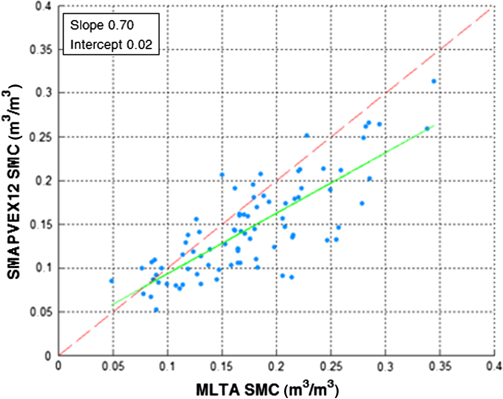
1.

Introduction

Soil moisture is a key environmental variable that influences a considerable number of geophysical processes, such as the water and carbon cycles. Its knowledge is, therefore, essential for several applications, such as drought and flood prediction and weather forecast. Moreover, soil moisture plays an important role in monitoring the effects of global climate change (e.g., droughts) and has very important implications for agriculture, ecology, and public health.

Volumetric soil moisture content (SMC) data can be directly measured by in situ probes, but ground stations provide punctual measurements, which are generally very sparse, so the spatial variability cannot be retrieved. Then, satellite remote sensing represents a very useful tool for monitoring soil moisture at different spatial and temporal scales, exploiting a direct sensitivity of microwave signals to SMC. In fact, in this spectral range, the soil dielectric permittivity is directly influenced by soil moisture, and the atmosphere can be considered fairly transparent.

Sensors operating in the low-frequency portion of the microwave spectrum (L-, C-band) are able to measure SMC within a suitable depth ($\sim 5\mathrm{cm}$ or shorter). However, the radar return is sensitive not only to soil moisture but also to surface roughness and, in the presence of vegetation, to the canopy structure and biomass. These effects make the retrieval process quite challenging. Nevertheless, these difficulties can be overcome through several approaches, such as multitemporal and change detection techniques.^1,2

Indeed, the multitemporal algorithms may mitigate these problems and deliver frequent and fairly accurate soil moisture maps, assuming that the variations of soil roughness and vegetation occur at longer temporal scales with respect to the soil moisture and the observations are taken within a short revisit time.^3,4

Soil moisture maps obtained from synthetic aperture radar (SAR) data are characterized by high spatial resolution, but SAR temporal resolution was generally considered a critical aspect for operational soil moisture applications. However, new SAR missions have been developed to provide data with short revisit time, such as the European Space Agency (ESA) Sentinel-1 (S-1)⁵ and the Soil Moisture Active/Passive (SMAP) mission of the National Aeronautics and Space Administration (NASA).⁶

A multitemporal algorithm⁷ [hereafter denoted as multitemporal algorithm (MLTA)] was initially conceived for deriving a soil moisture product from the data provided by the C-band S-1 mission, characterized by short revisit time (the two-satellite constellation offers 6 days repeat or less over Europe and Canada⁸). Considering the launch of the SMAP mission, operating in a frequency range (L-band) particularly suited for SMC applications, the MLTA has been adapted to work at L-band and to take advantage of the multipolarization (HH, VV, and HV) capability of SMAP. Unfortunately, the SMAP radar stopped operating at the beginning of July 2015; nevertheless, a few months of radar data acquisitions can be exploited to assess its potential for high spatial and temporal resolution SMC mapping in view of future L-band missions, such as the Argentinian SAOCOM.

This paper presents the work performed to adapt the forward models used in the MLTA to multipolarization measurements at L-band. The simple Oh and Sarabandi Model⁹ is proposed to simulate the bare soil backscattering at L-band. Indeed, in this case study, when compared with the SAR measurements, the bare soil backscattering produced by the model showed an error trend dependent on the soil moisture and roughness of the analyzed fields. Moreover, different approaches were investigated to separate the soil backscattering contribution from that of the canopy; indeed, depending on the structure of the plants, it was possible to consider simple scattering terms or to take into account additional factors, as the soil–vegetation interactions. In both cases, the normalized difference vegetation index (NDVI) was used to represent the state of vegetation. The outcomes of a preliminary test of the MLTA soil moisture retrieval based on L-band data are presented here.

This work was accomplished taking advantage of the availability of the data from the SMAP validation experiment 2012 (SMAPVEX12) campaign consisting of L-band radar images collected by the uninhabited aerial vehicle synthetic aperture radar (UAVSAR) sensor, which is an aircraft-based, fully polarimetric radar implemented on the NASA Gulfstream-III aircraft, as well as in situ SMC and vegetation data. The results of the inversion algorithm, summarizing the strengths and weaknesses of the approach, are presented.

2.

SMAP Validation Experiment 2012 Campaign

The SMAPVEX12 (Ref. 10) is a field campaign established to provide data for algorithm evaluation and testing in the frame of the SMAP mission. The campaign has been carried out in an agricultural region south of Winnipeg, Manitoba (Canada) from June 6 to July 7, 2012, where different crop types (such as corn, pasture, wheat, and soybeans) were present. For this experiment, coincident airborne and in situ data were acquired using both active and passive instruments:

The PALS instrument provides both radar products (including normalized radar cross section in HH, HV, VH, and VV) and radiometer data (including brightness temperature at vertical and horizontal polarization). The UAVSAR is an aircraft-based fully polarimetric L-band radar installed on the NASA Gulfstream-III aircraft. During the campaign, 13 UAVSAR flights were carried out, collecting data from an altitude of 13 km over a swath ($\sim 21\mathrm{km}$) between 20 deg and 65 deg of incidence angle. Only data collected between $\sim 35\mathrm{deg}$ and 45 deg were considered; then, the raw UAVSAR data were normalized to an incidence angle of 40 deg (the one of SMAP) using the histogram method.¹¹ For this study, the data provided by the UAVSAR with a spatial resolution of $5\mathrm{m}\times 7\mathrm{m}$ were used to tune and validate the forward models. The ground measurements of soil moisture were taken together with other surface characteristics close to the time of the airborne acquisitions. In general, multiple-location sampling is required to capture a significant representation of field average moisture. For this purpose, 16 measurements of soil moisture were sampled for every field, with three replicate measurements at each sample point. These 16 sample points were arranged in two transects of eight points with a distance of 200 m, while the points were 75 m apart; the surface covered by the measures was around $600\mathrm{m}\times 300\mathrm{m}$ for each field. Moreover, the measurements were taken 100 m from the field edges. As known, backscattering is also influenced by the soil roughness; this parameter was measured once early in the campaign at two sites in each field. Considering agricultural fields, the roughness is primarily due to land management activities, and since the campaign began after seeding, further effects were not expected. As for vegetation parameters, some static vegetation proprieties (such as plant density) were measured only once, while dynamic proprieties (such as biomass and canopy water content, phenology, etc.) were repeatedly monitored. More details about the acquisition strategy and the SMAPVEX12 data can be found in Ref. 10.

In this work, the 16 soil moisture measurements per day were averaged to have a soil moisture value representative of each field, and a shapefile indicating the position of every soil moisture measurement was used to properly average the SAR backscattering pixels pertaining to each field.

3.

Multitemporal Algorithm

The MLTA was designed in the framework of the “GMES Sentinel-1 Soil Moisture Algorithm Development” project⁷ funded by ESA (ESA Contract No. SMAD-TN-ACS-GS-0308). The proposed approach consists of retrieving soil moisture from a sequence of SAR acquisitions using a multitemporal Bayesian decision criterion [maximum a posteriori probability(MAP)], integrating a dense time series of radar backscatter measurements. The MLTA flowchart is depicted in Fig. 1.

Fig. 1

Processing chain of the MLTA.

The algorithm is based on the hypothesis that the temporal scale of variation of roughness is slower than that of soil moisture, i.e., considering a temporal interval in which a number of images are available, the average characteristics of surface roughness are not changing substantially, as opposed to soil moisture.

The MAP estimator inverts a forward soil backscattering model relating the backscattering coefficient to the bare soil parameters: not only soil moisture, but also soil roughness. The previous version of the MLTA software used the semiempirical Oh and Sarabandi model.⁹

Referring to a general polarimetric radar configuration, the surface target scattering is described by a polarimetric covariance matrix $\mathbf{C}$, whereas the radar supplies its estimate $\mathbf{Z}$, which differs from the target covariance matrix $\mathbf{C}$ because of observation uncertainties. The MAP estimator maximizes the probability density function (pdf) $p(\mathbf{\Theta }|\mathbf{Z})$ of the vector of soil parameters $\mathbf{\Theta }$ (i.e., moisture, roughness standard deviation, and correlation length) conditioned to the measurement vector $\mathbf{Z}$ (i.e., the radar observations at different polarizations and different times).

Considering the availability of a temporal series of measurements acquired at the current time $t$ and at $M$ previous times $t-M,\dots ,t-1$, the pdf to be maximized is

Regarding the effect of vegetation, several models were considered to separate the soil contribution from the canopy return.¹⁵ Here, the effects of vegetation on the radar signal are taken into account by applying semiempirical models of scattering from vegetation canopy. It is assumed that a simple semiempirical model may be better adapted to the data and encompasses a larger range of vegetation types by a proper parameter tuning. Nevertheless, simple models that consider only single scattering terms¹⁶ can be suitable when the vegetation is not very much developed. For some kinds of crops, and even at L-band, the forward model may require a correction to take into account other scattering sources, such as the interaction between the soil and the vegetation, as will be discussed later on.

4.

Retrieval of Bare Soil

4.1.

Forward Model Tuning

Among several algorithms present in the literature to simulate the backscattering from bare surfaces, two models were analyzed: a semiempirical model (the Oh and Sarabandi⁹) and an algorithm based on the method of moment [the 3-D numerical method of Maxwell’s equations (NMM3D)],¹⁷ whose output is made available in a look-up table and described in Ref. 18.

The two models were compared over bare soils, which were selected from the SMAPVEX12 fields using a threshold on the vegetation water content (VWC), i.e., VWC measured on the ground $<0.5\mathrm{kg}/{\mathrm{m}}^2$.¹⁹ The fields selected for this analysis were those numbered as 21-23-24-52-64-82, which span several soil characteristics, including different cultivations. Indeed, the fields were representative of pasture, corn, and soybean and have been worked in different ways, thus producing different roughness.

The results of the comparison between the modeled and measured backscattering are shown in Fig. 2, where the colors represent the different polarizations (blue and red for the HH and VV polarizations, respectively).

Fig. 2

Comparison between modeled and measured backscattering coefficient for HH (cyan dots) and VV (red dots) polarizations. (a) and (b) refer to the Oh and Sarabandi and NMM3D simulations. Green line represents the perfect alignment.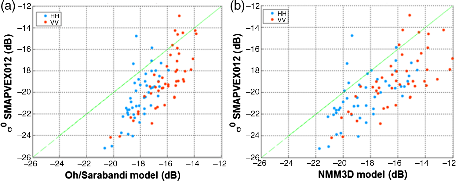

In such analysis, the Oh and Sarabandi model presents slightly better performances in terms of correlation coefficient and root mean square difference (RMSD) compared with to the NMM3D method, as reported in Table 1. Then, it has been selected to simulate the bare soil backscattering at L-band.

Table 1

Scores of the matching between the measured backscatter and those provided by the Oh and Sarabandi (columns 2 and 3) or NMM3D model (columns 4 and 5).

	Oh and Sarabandi		NMM3D
	R (#)	RMSD (dB m3 m−3)	R (#)	RMSD (dB m3 m−3)
HH	0.68	2. 29	0.61	2.71
VV	0.79	3.21	0.71	3.36

Nevertheless, analyzing the error between the simulated and measured backscattering as a function of soil moisture and roughness, it has been possible to highlight its dependence on these latter variables. Such dependence is particularly evident when the error is plotted as a function of soil moisture (upper row of Fig. 3).

Fig. 3

Difference between the backscattering coefficient simulated by the Oh and Sarabandi model and the measured ones for (a) HH, (b) VV, and (c) HV polarizations. The upper figures show the error as a function of soil moisture and the lower ones as a function of soil roughness. The green line represents the best fitting line, and its slope and RMSE are reported in the legend.

The correlation coefficients between backscattering model error and measured soil moisture (or soil roughness) are $-0.62$ (0.16) for HH, $-0.50$ (0.10) for VV, and $-0.15$ (0.21) for HV polarization, with best fitting line parameters reported in Fig. 3. A first-degree empirical polynomial factor, dependent on soil roughness standard deviation $s$ (cm) and soil moisture SMC (${\mathrm{m}}^3{\mathrm{m}}^{-3}$) according to Eq. (5), has been fitted for each polarization to reduce the error in decibel between the modeled and measured data at all polarizations

Eq. (5)

$${\sigma }_{\mathrm{mod}}^0-{\sigma }_{\mathrm{meas}}^0=a+b·\mathrm{SMC}+c·s.$$

The fitting has been performed using a MATLAB^© fitting script, which minimizes the RMSD in the equation. The Oh and Sarabandi model is an empirical model. As such, its performances are functions of the statistical significance of the training set used to fit the model to the data. A comparison between the Oh modeled and measured backscatter was also performed in Wang et al.,²⁰ where Radarsat-2 was considered. In that work, an overestimation of the modeled backscattering with respect to the measurements was observed, and this is confirmed by the results shown in Fig. 3. The decrease of such overestimation for increasing soil moisture, observed in Fig. 3, indicates an earlier saturation of the modeled backscatter with respect to the measured one at L-band and 40 deg of incidence angle. The simple correction of the Oh model proposed here at L-band aims at reducing the overestimation and at the same time increasing the sensitivity in the high range of soil moisture.

Then, using Eq. (5) with the retrieved coefficients $a$, $b$, and $c$, a modified Oh and Sarabandi model, with error independent on the soil characteristics, was obtained. The model tuning was cross-validated through the leave one-out (LOO) technique. According to this approach, the model fitting is carried out by including all the data minus one; then, the distance between the modeled and measured backscattering is evaluated for the excluded point. This procedure is repeated for all the experimental points; then, the RMSD of all distances is evaluated. From this analysis, a correlation coefficient of 0.82 and an RMSD around 1.4 dB were found; the results are reported in Fig. 4.

Fig. 4

Comparison between the measured backscattering coefficient and modeled ones (derived from the LOO analysis) using the modified Oh and Sarabandi model. (a) HH, (b) VV, and (c) HV polarizations. The green line represents the best fitting line, and its slope and intercept values are reported in the legend.

Then, considering that in the retrieval algorithm only one forward model is required and the differences of RMSD values using the LOO technique and that obtained using coincident training and testing points were negligible, the final forward model was estimated using the whole set of data points. The three coefficient $(a,b,c)$ values were (5.86 dB, $-16.99\mathrm{dB}/{\mathrm{m}}^3{\mathrm{m}}^{-3}$, $-0.54\mathrm{dB}/\mathrm{cm}$) for HH, (6.13 dB, $-14.65\mathrm{dB}/{\mathrm{m}}^3{\mathrm{m}}^{-3}$, $-0.70\mathrm{dB}/\mathrm{cm}$) for VV, and ($-0.23\mathrm{dB}$, $-3.01\mathrm{dB}/{\mathrm{m}}^3{\mathrm{m}}^{-3}$, $1.26\mathrm{dB}/\mathrm{cm}$) for HV polarizations, respectively. The comparison between the model and data showed a correlation degree around 0.84 and an RMSD of 1.35 dB. Even if the correction of the sensitivity of the Oh model to soil roughness is quite small, a slight worsening of the root mean square error of the corrected model can be noticed without roughness correction, which is detrimental for soil moisture retrieval, as shown later on.

4.2.

Retrieval Results

The MLTA has been preliminarily tested on bare soil fields, using the forward model tuned, as previously described. The bare fields have been chosen among the SMAPVEX12 data imposing a threshold on the VWC as before.

During the campaign timeframe, 11 acquisitions were considered over the considered fields and the MLTA software was run with a temporal frame equal to 5, i.e., looking at four images behind. The comparison between the retrieved and the measured soil moisture is reported in Fig. 5, where it is possible to note that the retrieval exhibits fairly good performances, with fairly high degree of correlation ($R=0.73$) and an RMSD of $0.045{\mathrm{m}}^3{\mathrm{m}}^{-3}$.

Fig. 5

Comparison between soil moisture retrieved by the MLTA and the measured ones over bare soils. Dashed red and green lines represent the perfect agreement and the best fitting lines, respectively. The slope and the intercept values of the best fitting line are reported in the legend.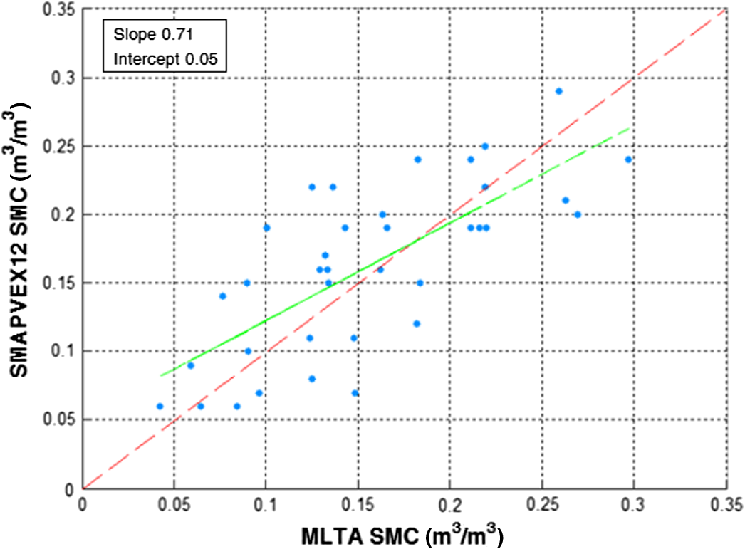

Note that directly using the Oh and Sarabandi model without the proposed empirical correction to simulate the bare soil backscattering, the retrieval algorithm results showed a correlation coefficient around 0.57 with an RMSD of $0.13{\mathrm{m}}^3{\mathrm{m}}^{-3}$. Moreover, as mentioned, the performances of the retrieval also worsened considering a model correction only based on the soil moisture, resulting in an RMSD of $0.06{\mathrm{m}}^3{\mathrm{m}}^{-3}$.

5.

Retrieval Over Vegetated Soil

In most of the works in the literature, soil moisture retrieval over vegetated surfaces is based on the water cloud model (WCM),¹³ which does not consider the multiple scattering contribution from vegetation–soil interaction, and models the canopy as a water cloud whose droplets are randomly distributed within the layer. For instance, the WCM was used by Dabrowska-Zielinska et al.²¹ to analyze the C- and L-band backscatter of several crops, such as wheat, grassland, and rape, showing a correlation coefficient between modeled and measured backscattering around 0.8. In Ref. 22, cropland L-band backscattering was also analyzed and modeled through WCM, presenting an RMSD around 3 dB for both HH and VV polarizations. An alternative method for soil moisture retrieval under canopy at C- and L-band was proposed by Joseph et al.²³ in which the ratio (indicated as RRI) of the bare soil and the measured backscattering was related to a vegetation parameter and then used to correct the canopy effects. Kim et al.¹⁸ proposed a soil moisture retrieval algorithm for SMAP radar data based on the inversion of a look-up table representation of a forward model (namely, a “datacube”). A very detailed scattering model was used to build the datacube, but only three input parameters were considered to query the look-up table, i.e., the VWC for vegetation and the soil dielectric constant and surface roughness.

In this work, the WCM and RRI models were used to predict the canopy backscattering, depending on the occurrence of single or multiple scattering within the canopy.

5.1.

Forward Model Tuning

The MLTA was tested over vegetated areas, independently analyzing each crop type present in the test area, in particular, corn, soybean, and wheat. Grouping the crops to use a common model to describe the interactions with the radar signal was attempted, but it was not possible due to the different plant structure. Indeed, grouping the crops, the modeled backscattering presented a high distance from the measured ones. In particular, the comparison between modeled and measured backscattering for both polarizations showed an RMSD around 3 to 3.5 dB using the two mentioned vegetation models, i.e., WCM and RRI, and merging all the data poins, regardless of plant category.

Starting with the wheat fields, the WCM was used to take into account the effects of the canopy, and it was tuned using the SMAPVEX12 data. The parameters of the WCM, which are represented by the system of Eq. (6), were estimated by an RMSD minimization using a MATLAB^© fitting script

Eq. (6)

$$\begin{gathered} {\sigma }_{\text{canopy}}^0={\sigma }_{\text{vegetation}}^0+{\tau }^2{\sigma }_{\text{soil}}^0, \\ {\sigma }_{\text{vegetation}}^0=Aw\cos (\theta )(1-{\tau }^2), \\ {\tau }^2=\exp [-2Bw/\cos (\theta )], \end{gathered}$$

where $w$ is the VWC, $\theta$ is the radar incidence angle, $\tau$ is the vegetation opacity, and $A$ and $B$ are the empirical parameters to be tuned. The procedure aimed at minimizing the RMSD between the soil backscattering derived from the measurements, through the inversion of the WCM, and that derived from ground soil moisture and roughness parameters, through the modified Oh and Sarabandi model.

For this purpose, the NDVI, provided by MODIS and defined as reported in Eq. (7), has been used as proxy of the canopy vegetation content

Eq. (7)

$$\mathrm{NDVI}=\frac{\mathrm{NIR}-\mathrm{VIS}}{\mathrm{NIR}+\mathrm{VIS}},$$

where NIR and VIS represent the spectral reflectance measurements in the near-infrared and visible (red) regions, respectively. The NDVI provided by MODIS is characterized by a resolution around 300 m, which is suitable for selecting at least one MODIS pixel to associate a NDVI value to the field. A shapefile with the position of the in situ soil moisture measurements was used to identify the area of interest and to collect the relevant NDVI pixels. It is worth mentioning that the fitting of the WCM model was also attempted using the measured cross-polarization backscattering coefficient, or a combination of the polarizations (i.e., the radar vegetation index), but the best fitting performance was obtained using the NDVI.

The model fitting was cross-validated through the LOO analysis. The results of the LOO fitting test are reported in Fig. 6, which represents the backscatter coefficients retrieved by the model and those measured by the SAR sensor, while the scores are reported in Table 2.

Fig. 6

Comparison between the measured soil backscattering and those obtained through the WCM over wheat fields. Dashed red and green lines represent the perfect agreement and the best fitting line, respectively. The slope and the intercept values of the best fitting line are reported in the legend. (a) HH and (b) VV polarizations.

Table 2

Correlation coefficient (R), RMSD, and bias between the backscatter coefficients derived from the measurements and the model for wheat fields.

	R (#)	RMSD (dB)	BIAS (dB)
HH	0.83	1.10	$-0.13$
VV	0.82	1.29	$-0.06$

At each iteration of the LOO cross-validation, the model parameters were very similar, so the final WCM model was tuned using the whole set of data points; the $A$ and $B$ model coefficients were estimated around 0.033 (0.003) and 0.072 (0.456) for HH (VV) polarization, respectively. The comparison between the measured soil backscattering and those obtained through the WCM showed a correlation coefficient around 0.86 (0.82) with an RMSD of 0.93 (1.28) dB for HH (VV) polarization. In the literature, most of the WCM’s at L-band use other parameters to characterize vegetation state, rather than NDVI (i.e., directly the VWC or the leaf area index). However, it is worth mentioning that the NDVI is more frequently and easily obtainable than the other vegetation indicators. For instance, Dabrowska-Zielinska et al.²¹ used the WCM to simulate L-band (HH, 35 deg) canopy radar backscatter; the model was fitted using the measured VWC as a vegetation indicator and the WCM coefficients were estimated around 0.01 and 0.04 for $A$ and $B$, respectively. Even if in this work the WCM was fitted using the NDVI as input, the model coefficient values were consistent with those obtained in Dabrowska-Zielinska et al.²¹ for the canopy and soil backscattering.

The WCM fed by MODIS NDVI has been integrated into the software to separate the soil contribution from the canopy return at each time, and the MLTA has been tested over wheat fields. It is worth mentioning that, during the period of analysis, the considered wheat fields presented a VWC measured on the ground between 1.4 and $4\mathrm{kg}/{\mathrm{m}}^{-2}$, which characterizes a well-developed canopy.

Generally, the soil moisture temporal trend of each field is fairly well reproduced, which is demonstrated by the high correlation coefficient between the retrieved and measured soil moisture (around 0.74). Figure 7 shows the temporal trend of the soil moisture retrieved by the algorithm (green line) and that measured by in situ probes (blue line) for the wheat field ID 31.

Fig. 7

Temporal trend of soil moisture retrieved by MLTA (green line) and that measured by in situ probes provided by the SMAPVEX12 campaign (blue line) for the wheat field number 31.

Nevertheless, considering the whole comparison (i.e., all the seven analyzed fields pooled together), the results are not extremely good in terms of RMSD, which is around $0.077{\mathrm{m}}^3{\mathrm{m}}^{-3}$. The comparison of overall retrieved and measured SMC is plotted in Fig. 8.

Fig. 8

Soil moisture retrieved by the algorithm and those measured over wheat fields. Dashed red and green lines refer to the perfect agreement and the best fitting line, respectively. The slope and the intercept values of the best fitting line are reported in the legend.

However, normalizing the data of each field to make the temporal variability of the retrieval have the same mean of the observations gives promising results. Namely, for each field, the mean value of soil moisture (retrieved by the algorithm and/or measured by in situ probes) was calculated and removed from the corresponding dataset. The results showed a correlation coefficient of 0.85, with an RMSD of about $0.05{\mathrm{m}}^3{\mathrm{m}}^{-3}$, as reported in Fig. 9.

Fig. 9

Comparison between MLTA and ground measurements soil moisture estimates after a normalization of the mean value in each field. Dashed red and green lines represent the perfect agreement and best fitting lines, respectively. The slope and the intercept values of the best fitting line are reported in the legend.

This result suggests that local effects on the scattering response of the targeted fields have to be carefully accounted for, a task that will be better investigated in future work. Over wheat fields, the algorithm retrievals showed slightly lower performances with respect to those obtained by Kim et al.²⁴ In that work, a correlation coefficient of 0.92 and an unbiased RMSD around $0.05{\mathrm{m}}^3{\mathrm{m}}^{-3}$ were observed comparing the retrieved and measured soil moisture over the SMAPVEX12 wheat fields.

As for soybean and corn crops, the fitting of the WCM did not provide satisfactory results, as the forward model need to take into account other backscattering mechanisms, such as the interaction between the soil and the vegetation.

To keep the model as simple as possible, in this work, the approach proposed by Joseph et al.²³ was used: the ratio between the soil and canopy measured backscattering was related to a few parameters describing the canopy conditions, which can be considered quite effective and easily available, such as the NDVI. Hereafter, the ratio will be indicated as ${\mathrm{RRI}}_{\mathrm{pp}}$, where the pp subscript represents the considered polarization.

For the SMAPVEX12 soybean field, the trend of the RRI for both the polarizations was analyzed as a function of the VWC, and it is reported in Fig. 10.

Fig. 10

Ratio between the soil, predicted from ground data using the corrected Oh and Sarabandi model, and the soybean measured backscattering as a function of the VWC measurements in situ. (a) HH and (b) VV polarizations.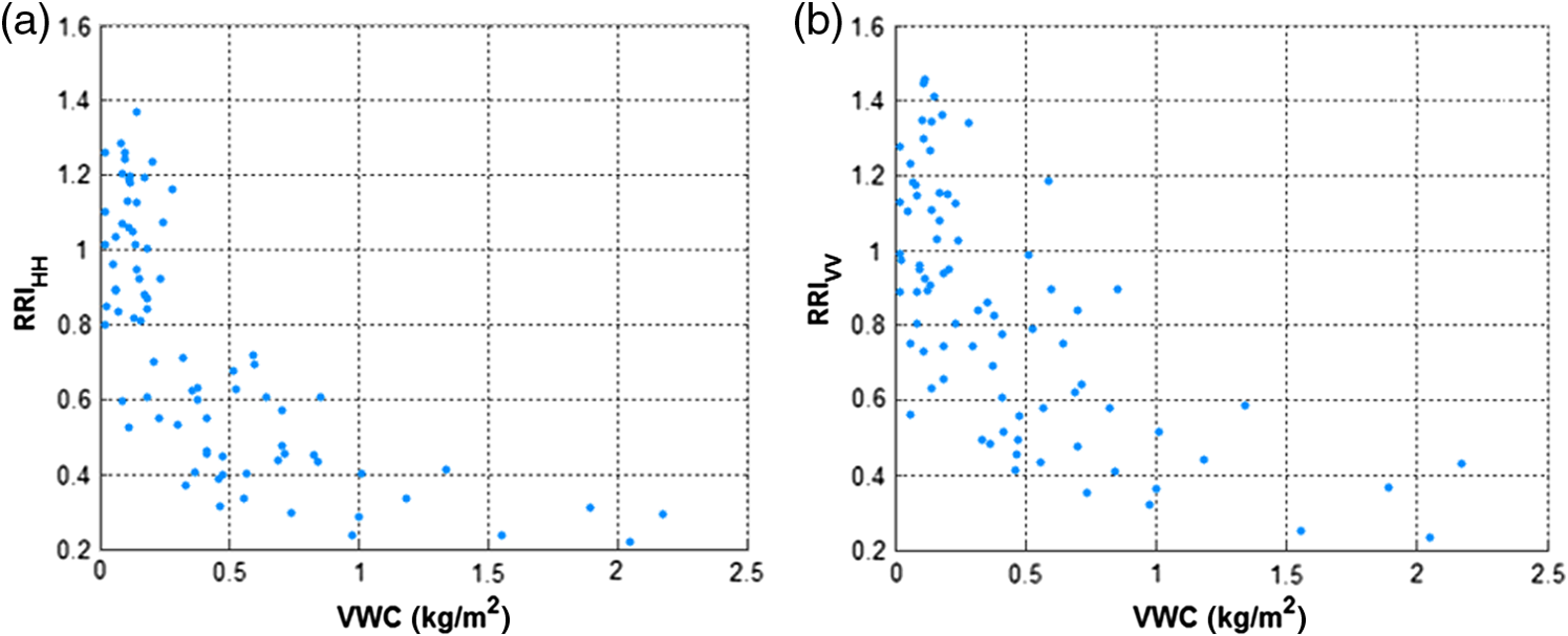

An exponential relationship between these parameters was observed and was fitted using the following Eq. (8) with parameters $A$ and $B$ tuned through a MATLAB^© script

Eq. (8)

$${\mathrm{RRI}}_{\mathrm{pp}}=A·\exp (-B·\mathrm{VWC}).$$

As done for the wheat fields, the empirical model used in the retrieval takes as input the NDVI provided by MODIS instead of the VWC measured on the ground. In Fig. 11, it is shown that the two parameters exhibit a nice exponential relationship, so the VWC is estimated from the NDVI using Eq. (9), whose parameters $a$ and $b$ were evaluated again through a MATLAB^© script minimizing the root mean square error

Eq. (9)

$$\mathrm{VWC}=a·\exp (-b·\mathrm{NDVI}).$$

Then, starting from the canopy backscattering and the NDVI provided by MODIS, it was possible to invert the exponential model to extract the soil backscattering contribution from the measured canopy radar return. The comparison between the soil contribution provided by the modified Oh and Sarabandi model, using the in situ measurements, and that derived using the Eqs. (8) and (9) through the LOO analysis showed encouraging results, as reported in Table 3 and in the scatterplot of Fig. 12.

Fig. 11

Comparison between the measured in situ VWC and the NDVI provided by MODIS over the SMAPVEX12 soybean fields. The green line represents the exponential fitting of Eq. (9).

Table 3

Correlation coefficient (R), RMSD, and bias between the backscatter coefficients of the soil contributions provided by the in situ measurements, using the modified Oh and Sarabandi model, and from the measured canopy backscattering using the empirical model for soybean fields.

	R (#)	RMSD (dB)	BIAS (dB)
HH	0.72	1.42	0.03
VV	0.81	1.47	0.19

Fig. 12

Comparison between the backscatter coefficients of the soil backscattering contributions provided by the in situ measurements, using the modified Oh and Sarabandi model, and that derived from the radar measurements using the adopted empirical model for RRI. Dashed red and green lines represent the perfect agreement and the best fitting lines, respectively. The slope and the intercept values of the best fitting line are reported in the legend.

Since the differences of RMSD values using the LOO technique and those obtained using coincident training and testing were negligible, all available data were considered to tune the forward model. The results showed a correlation coefficient around 0.73 (0.81) with an RMSD of 1.37 (1.44) dB for HH (VV) polarization. After performing the vegetation correction, the MLTA results over the soybean fields showed good performances, as reported in Fig. 13; the temporal trend of soil moisture was well-reproduced, showing a degree of correlation around 0.75 and an RMSD of $0.05{\mathrm{m}}^3{\mathrm{m}}^{-3}$. Over soybean fields, the algorithm retrievals showed a correlation coefficient similar to that evaluated by Kim et al.²⁴ with an improvement of the RMSD; in Ref. 24, an unbiased RMSD around $0.09{\mathrm{cm}}^3{\mathrm{cm}}^{-3}$ was observed.

Fig. 13

Comparison between the retrieved and in situ measured soil moisture over soybean crops. Dashed red and green lines represent the perfect agreement and the best fitting lines, respectively. The slope and the intercept values of the best fitting line are reported in the legend.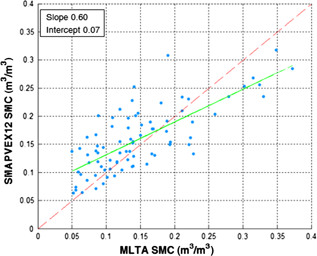

A similar approach has also been applied to the corn fields. As previously done, the soil contribution was extracted using the canopy backscattering and the information related to the vegetation growing, as reported in Fig. 14.

Fig. 14

Ratio between the soil backscatter predicted from ground data using the corrected Oh and Sarabandi model, and the corn measured backscattering as a function of the VWC measurements in situ. (a) HH and (b) VV polarizations.

In this case, the comparison between the real and the derived soil backscatter through the LOO analysis is plotted in Fig. 15, while the evaluated performances of the model are reported in Table 4.

Fig. 15

Comparison between the backscatter coefficients of the soil backscattering contributions provided by the in situ measurements, using the modified Oh and Sarabandi model, and that derived from the radar measurements using the adopted empirical model for RRI over corn crops. Dashed red and green lines represent the perfect agreement and the best fitting lines, respectively. The slope and the intercept values of the best fitting line are reported in the legend.

Table 4

Correlation coefficient (R), RMSD, and bias between the backscatter coefficients of the soil contributions derived from the in situ measurements, using the modified Oh and Sarabandi model, and from the model for corn fields.

	R (#)	RMSD (dB)	BIAS (dB)
HH	0.78	1.34	$-0.27$
VV	0.86	1.18	0.03

Throughout the LOO analysis, the estimated model coefficients remained in a short range; then, the whole set of data points was used to tune the forward model. The results showed a correlation coefficient of 0.78 (0.85) with an RMSD of 1.18 (1.15) dB for HH (VV) polarization.

When testing the MLTA over the corn fields, the comparison between the retrieved and measured soil moisture showed a correlation degree of 0.8 and a root mean square of about $0.048{\mathrm{m}}^3{\mathrm{m}}^{-3}$. Over corn fields, the algorithm retrievals showed good performances with respect to those obtained by Kim et al.,²⁴ who obtained an unbiased RMSD around $0.05{\mathrm{cm}}^3{\mathrm{cm}}^{-3}$ and a correlation coefficient of 0.66. The trend of the comparison is shown in Fig. 16.

Fig. 16

Comparison between the retrieved and in situ measured soil moisture over corn fields. Dashed red and green lines represent the perfect agreement and the best fitting line, respectively. The slope and the intercept values of the best fitting line are reported in the legend.

6.

Discussions

This work demonstrates that models to correct vegetation effects and retrieve soil moisture in agricultural areas must be adapted to the different crop types. However, simple semiempirical models are suitable and provide quite good performances. In general, in the considered study area, the growing season was relatively short, starting from the seeding in April/May to the harvesting on August/September. For the wheat fields used in our analysis, the VWC presented values between 1 and $4\mathrm{kg}/{\mathrm{m}}^2$, representative of plants already well-developed. It was confirmed that the WCM was suitable to correct the effect of wheat plants, until maturity, where single scattering and attenuation are the main interaction mechanisms. For soybean and corn fields, the period of analysis covered the whole plant development, presenting values of VWC from 0 to $3.6\mathrm{kg}/{\mathrm{m}}^2$. To account for multiple scattering mechanisms involved for these crop types, the RRI method, although purely empirical, outperformed other approaches, such as adding a double bounce scattering mechanism to the WCM. Another important issue is how to retrieve the vegetation growing stage. From an electromagnetic point of view, the VWC is the most effective input parameter. However, in practice, a suitable proxy needs to be selected if we want to rely on easily available information. Although it is generally observed that the NDVI tends to saturate for well-developed vegetation, it provided better vegetation correction compared to radar based index. The latter are likely affected by other parameters, such as soil conditions.

These outcomes have a general validity and can be extended to other types of crops once a training experimental data set is available. Even if the SMAP radar acquisitions are quite limited due to the radar failure, this work is of interest for the analysis of backscattering images provided by a generic radar operating at L-band (as for instance the Argentinian SAOCOM²⁵ mission), for which the semiempirical models proposed here could be used, provided the different incidence angle is taken into account.

7.

Conclusions

In this study, a semiempirical backscattering model for bare surfaces has been analyzed and modified to retrieve soil moisture at L-band through a MLTA. The SMAPVEX12 experiment was used for this purpose, providing images collected by the UAVSAR, and the ground survey. In bare soil conditions, the MLTA showed fairly good performances (RMSD of about 4.5%). For the vegetated fields, simple semiempirical backscattering models were considered and updated using the SMAPVEX12 data over the main surveyed crops to single out the soil backscattering contribution from that of the canopy. As for wheat fields, the WCM was calibrated, obtaining a value of 0.033 (0.003) for the canopy attenuation and of 0.072 (0.456) for canopy scattering, considering the HH (VV) polarization. For soybean and corn, where the soil–canopy interaction may be important, an empirical- and crop-dependent exponential model was set up using the NDVI as a proxy for the VWC. For soybean fields, the values for the scaling and exponential factor were 1.01 (1.19) and 0.88 (0.66) for HH (VV) polarization, whereas for the corn crop, they were 1.05 (0.67) and 0.75 (0.54) for HH (VV) polarizations. The results showed an RMSD of the retrieval in the order of 5% for the soybean and corn crops, whereas for wheat, some unexplained biases among different fields were observed. If those biases are removed, the results in terms of RMSD go down from 7.7% to 5%.

The described approach is being tested on the data collected by the SMAP mission, which, in spite of the failure of the instrument, has collected a significant amount of radar data worldwide.