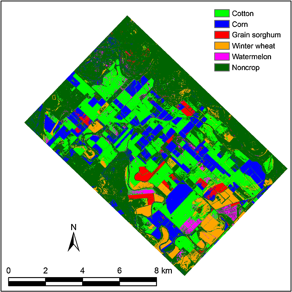
1.

Introduction

The boll weevil (Anthonomus grandis grandis Boheman) is now eradicated from all cotton-producing states in the U.S. except for the Rio Grande Valley of Texas.¹ However, the cotton (Gossypium hirsutum L.) growing areas, especially those adjacent to the lower Rio Grande Valley, will remain susceptible to reinfestation from boll weevils that migrate or are transported on cotton harvesting equipment. The eradication program functions by monitoring all cotton fields using pheromone traps to detect incipient weevil populations and by applying insecticides when and where justified by weevil captures or as preventive measures.² Although cotton producers are required to report the location of planted cotton fields to the Farm Service Agency, this information is belatedly available for the boll weevil eradication program. Therefore, early identification of fields planted in cotton is critical for eradication program managers to effectively monitor boll weevil populations and treat the respective fields in a timely manner.

Another important aspect to ensure the success of the eradication program is the mandatory and timely elimination of cotton plants following harvest and the subsequent creation of a host-free period. By law, cotton plants must be destroyed after harvest by a certain date to prevent regrowth of cotton fruit on which weevil populations can survive and reproduce.³ Volunteer cotton plants can also germinate from seed that remains in a field after harvest or that is inadvertently scattered by floods or by transport of harvested cotton to gins. Information on the location and area of planted cotton fields will facilitate the quick detection of potential areas for volunteer and regrowth cotton plants.

Multispectral imagery from satellite sensors, such as Landsat and SPOT, has been used for crop identification and area estimation for decades.^4–7 As high-resolution satellite sensors, such as IKONOS, QuickBird, and SPOT 5, have become available more recently, imagery from these sensors has also been evaluated for crop identification.^8–12

Recent advances in imaging technologies have made consumer-grade digital cameras an attractive option for remote sensing applications due to their low cost, small size, compact data storage, and ease of use. Consequently, consumer-grade digital color cameras have been increasingly used by researchers for agricultural applications.^13–16 Unlike traditional sophisticated airborne imaging systems that need to be mounted on designated remote sensing aircraft, imaging systems based on consumer-grade cameras can be easily mounted on any small aircraft with no or minimal modification.¹⁷ Furthermore, agricultural aircraft provide a readily available and versatile platform for airborne remote sensing. Single-camera and two-camera imaging systems have been attached to agricultural aircraft to take aerial images for monitoring crop growing conditions and detecting crop pests.^15–18

Since aerial imagery has a relatively small ground coverage compared with satellite imagery, a large number of images taken along multiple flight lines with specified minimum overlaps are needed to cover a large geographic region. Image mosaicking techniques are then used to mosaic the images. Most image processing software, such as Erdas Imagine (Intergraph Corporation, Madison, Alabama), requires that the input images be georeferenced to a coordinate system with known projection information before being mosaicked based on their geographic position. Another approach for image mosaicking is based on the content of the images using photogrammetry software, such as Pix4DMapper (Pix4D SA, Lausanne, Switzerland). Pix4DMapper can automatically convert large numbers of aerial images into georeferenced two-dimensional orthomosaics and three-dimensional surface models using the latest innovations in computer vision and photogrammetry.

Various pixel-based classification methods have been used to classify remote sensing imagery. These include traditional unsupervised and supervised classification methods, such as iterative self-organizing data analysis and maximum likelihood (ML), as well as more advanced techniques, such as artificial neural networks, support vector machines, and decision trees.^19–22 These classifiers and techniques provide varying levels of success for crop identification depending on the complexity of crop growing environments. However, with the pixel-based classification approach, pixels are classified individually based on their spectral characteristics regardless of their spatial aggregation. Another approach for crop identification is object-based classification, which typically relies on segmentation algorithms to define geographical objects that can be classified. Object-based classification can improve classification accuracy.^23,24 Therefore, object-based techniques have been increasingly used for image classification.^25–27 However, object-based classification generally requires additional software and advanced image processing skills.^16,28 For parcel- or field-based classification, field boundaries need to be available or manually digitized.^12,24 This can add more processing time and cost for the production of classification maps.

The overall goal of this study is to develop practical methodologies for early identification of cotton fields using airborne multispectral imagery. To achieve this goal, accurate and easy-to-use image mosaicking and classification techniques needed to be identified for efficient and quick implementation. As discussed above, satellite imagery has been widely used for crop identification, but limited work has been reported on early identification of cotton fields, especially using aerial imagery. Therefore, the specific objectives of this study are to: (1) evaluate position- and content-based image mosaicking techniques for creating mosaics from overlapped aerial multispectral imagery; (2) compare five commonly used supervised classification methods, including ML, minimum distance (MD), Mahalanobis distance (MAHD), spectral angle mapper (SAM), and spectral correlation mapper (SCM), for crop identification from the mosaics; and (3) identify practical image mosaicking techniques and classification methods that can be easily implemented for identification of cotton fields from aerial imagery before cotton plants begin to flower.

2.

Materials and Methods

2.1.

Study Site

An $8\mathrm{km}\times 12\mathrm{km}$ cropping area with the center coordinates (30°34′11″N, 96°29′4″W) along the Brazos River near Snook, Burleson County, Texas, was selected for this study (Fig. 1). The soils in the area are very deep and very slowly permeable with slopes ranging from 0% to 3%. The surface layer and subsoil are reddish brown clay underlain by dark gray silty clay loam. The underlying material is mainly composed of clayey and loamy alluvial sediments. The clayey surface layer may delay cultivation after periods of prolonged rainfall. Cotton, corn, and grain sorghum are the main crops. Minor crops, such as winter wheat, soybeans, watermelon, and alfalfa, are also cultivated. Corn and grain sorghum are typically planted in February to March and harvested in July to August, while cotton is planted in April to May and harvested in August to October. In the 2014 growing season, cotton and corn were the two main crops, while grain sorghum, winter wheat, and watermelons were grown in the study area. Other noncrop cover types included mixed herbaceous species (pasture), lush grass (hay), mixed woody species, water bodies, and bare soil/impervious surfaces.

Fig. 1

An $8\mathrm{km}\times 12\mathrm{km}$ cropping area (yellow box) near Snook, Texas, with geotagged RGB images (thumbnails) plotted along two flight lines on Google Earth. The thumbnails just represent the image locations but not the actual image sizes.

3.

Results and Discussion

Figures 2 and 3 present the mosaicked CIR images from the 32 pairs of RGB and NIR images using the position- and content-based approaches, respectively. Visually, the two mosaics look very similar. However, mismatches and color differences around overlapped areas in the position-based mosaic are noticed when the image was enlarged, while no mismatch or artifact is found in the content-based mosaic. Both mosaics reveal distinct differences among the crops and other cover types in the study area. On the CIR images, crops and other vegetation generally had a reddish color. Since corn and grain sorghum were at their peak growth, they had a dark red tone. Cotton plants were relatively small and there was substantial soil exposure, so cotton fields had a pinkish tone. Winter wheat was mature and some fields were even harvested, so it had a gray to dark gray color. There were only a few watermelon fields, and they had a magenta color.

Fig. 2

Mosaicked CIR image from 32 pairs of RGB and NIR images using the position-based approach with no color correction and the feather overlay function in Erdas Imagine.

Fig. 3

Mosaicked CIR image from 32 pairs of RGB and NIR images using the content-based approach in Pix4DMapper.

Figures 4 and 5 show the six-class classification maps generated from the two respective mosaics presented in Figs. 2 and 3 based on the ML classifier. Although the AGGIE-GIS aggregation was applied to the classification maps, many small areas greater than $10\mathrm{m}\times 10\mathrm{m}$ can be seen in the maps. A quick comparison with the CIR images indicates that the classification maps provided good separations among the crops and the noncrop class. Most of the fields on the classification maps had only one dominant class, but all fields contained small inclusions of other classes due to the within-field variability and spectral similarities among some of the classes.

Fig. 4

ML-based classification map for the position-based mosaic shown in Fig. 2.

Fig. 5

ML-based classification map for the content-based mosaic shown in Fig. 3.

Table 1 summarizes the accuracy assessment results for the 40 classification maps generated from the position-based mosaics. Overall accuracy ranged from 64.7% for the 10-image mosaic created using the color balancing and the simple overlay and classified with the SCM classifier to 90.4% for the 32-image mosaic created using no color correction and the feather overlay and classified with the ML classifier. These accuracy values indicated that 65% to 90% of the pixels in the study site were correctly identified in the 40 classification maps using the five classification methods. Overall kappa ranged from 0.508 to 0.860 among the 40 classification maps. Kappa values indicate how well the classification results agree with the reference data. A kappa value of 0 corresponds to a total random classification, while a kappa value of 1 represents a perfect agreement between the classification and reference data.

Table 1

Classification accuracy assessment results for mosaicked images created from georeferenced four-band images using different combinations of color correction methods and overlay functions for a cropping area.

Among the five classifiers, ML performed better than any of the other four classifiers for all the eight mosaics. MAHD was superior to the other three classifiers in all cases except in one case where MD was better and in two cases where SAM was better. MD had similar performance to SAM, while SCM was the worst among the five classifiers. Between the two overlay functions, the feather function was better than the simple overlay. Among the three color correction methods, no color correction appeared to be better than color balancing or histogram matching, although the differences among the three were marginal. The overall accuracy values using all 32 images were slightly higher than those using only 10 images for three of the four color correction and overlay function combinations. Based on these results, ML applied to either the 10-image or 32-image mosaic created using no color correction and the feather overlay function produced the best classification maps.

Table 2 summarizes the accuracy assessment results for the five classification maps generated from the content-based mosaics. Similarly, ML performed best, and SCM had the lowest overall accuracy and overall kappa values among the five classifiers. The best overall accuracy was 91.3% for the four-band mosaic, slightly higher than the best overall accuracy for the position-based four-band mosaic (90.4%). The advantage of the NIR band is clearly seen from the difference in overall accuracy between the four-band mosaic and the RGB composite (91.3% versus 83.8%, respectively). The CIR or NIR–red-green composite had a similar overall accuracy to that of the four-band mosaic. It also had the highest overall accuracy among the four three-band composites, indicating that a single CIR camera is as effective as the combination of an RGB and an NIR camera.

Table 2

Classification accuracy assessment results for mosaicked four-band and three-band images created from 32 pairs of RGB and NIR images using the content-based approach for a cropping area.

As overall accuracy indicates the overall performance of all classes as a whole in a classification map, producer’s and user’s accuracies are more meaningful for the individual classes. Producer’s accuracy of a class indicates the probability of actual areas for that class being correctly classified, and user’s accuracy of a class indicates the probability that areas classified as that class on the map actually represent the class on the ground. Tables 3 and 4 present the error matrices and accuracy measures for the ML-based classification maps for the position-based four-band mosaic and the content-based four-band mosaic, respectively. Producer’s accuracy varied from 79% for grain sorghum to 97% for winter wheat for the position-based mosaic and from 86% for watermelon and grain sorghum to 97% for winter wheat for the content-based mosaic, whereas user’s accuracy ranged from 75% for winter wheat to 95% for noncrop for the position-based mosaic and from 79% for grain sorghum to 95% for noncrop for the content-based mosaic. The content-based mosaic had slightly higher overall accuracy and kappa values than the position-based mosaic.

Table 3

An error matrix and accuracy measures for an ML-based classification map for a mosaicked four-band image created from 32 manually georeferenced images with no color correction and the feather overlap function for a cropping area.

Table 4

An error matrix and accuracy measures for an ML-based classification map for a four-band mosaic created from 32 pairs of RGB and NIR images using the content-based approach for a cropping area.

For the position-based mosaic, cotton had a producer’s accuracy of 88.0% and a user’s accuracy of 91.4%. These values indicate that 88% of the cotton areas on the ground were correctly identified as cotton, whereas 91% of the estimated cotton areas on the classification map were actually cotton. In other words, the classification map missed 12% (omission error) of the cotton areas on the ground, while about 9% (commission error) of the pixels classified as cotton on the classification map actually belonged to the other classes. Of the 276 points verified on the ground as cotton, 5 points (1.8%) were misclassified as corn, 6 (2.2%) as winter wheat, 12 (4.3%) as watermelon, and 10 points (3.6%) noncrop on the classification map. On the other hand, of the 266 points classified on the classification map as cotton, 2 (0.8%), 1 (0.4%), and 20 points (7.5%) were actually corn, grain sorghum, and noncrop, respectively. The producer’s and user’s accuracies for corn and noncrop were better than those for the other crops. It should be noted that some of these misclassifications were due to the small inclusions in the dominant class. If the whole field was considered as one unit, the classification accuracy would improve. For the other classes, winter wheat had a high producer’s accuracy of 97% and a low user’s accuracy of 75%. This indicates that although 97% of the winter wheat areas on the ground were correctly identified as winter wheat, only 75% of the areas called winter wheat on the classification map were actually winter wheat. In other words, winter wheat areas on the classification map overestimated the actual winter wheat areas.

For the content-based mosaic, the producer’s and user’s accuracies for cotton were both close to 91%, indicating 91% of the cotton areas on the ground were correctly identified as cotton and 91% of the areas called cotton on the classification map were actually cotton. Of the 276 points verified on the ground as cotton, 2 points (0.7%) were misclassified as corn, 6 (2.2%) as winter wheat, 3 (1.1%) as watermelon, and 14 (5.1%) as noncrop on the classification map. Moreover, of the 277 points classified as cotton on the classification map, 2 points (0.7%) actually belonged to corn, 1 (0.4%) to grain sorghum, 1 (0.4%) to watermelon, and 22 (7.9%) to noncrop. Similarly, the producer’s and user’s accuracies for corn and noncrop were generally better than those for the other crops.

Tables 5 and 6 give area estimates of cotton and noncotton classes from the ML-based classification maps for the eight position-based mosaics and the five content-based mosaics. The eight position-based mosaics provided very similar area estimates for cotton, ranging from 2220 to 2454 ha or 23.0% to 25.4% of the total area, although the four position-based mosaics using all 32 images provided slightly higher estimates than those using only 10 images. In practice, using only 10 images can significantly reduce the time required for image alignment and georeferencing. The area estimates for cotton based on the content-based four-band mosaic, the CIR composite, and the RGB composite (24.7% to 25.4%) were similar to those based on the position-based mosaics. However, the estimates based on the NIR-red-blue and NIR-green-blue composites (21.4% and 21.0%) were 3% to 4% lower. As different classification maps had varying overall accuracy values as well as producer’s and user’s accuracy values, the variation in area estimates was expected.

Table 5

Area estimates of cotton and noncotton classes from ML-based classification maps for mosaicked images created from georeferenced four-band images using different combinations of color correction methods and overlay functions for a cropping area.

Table 6

Area estimates of cotton and noncotton classes from ML-based classification maps for mosaicked four-band and three-band images created from 32 pairs of RGB and NIR images using the content-based approach for a cropping area.

The best position-based mosaic created from all 32 images using no color correction and the feather overlay function provided an area estimate of 2424 ha or 25.1% for cotton. In comparison, the best content-based four-band mosaic provided a very similar area estimate of 2453 ha or 25.4%. These numbers could be used as the best estimates for cotton. It should be noted that although it is important to estimate the cotton production area, it is more important to identify cotton fields for the boll weevil eradication program. Considering the small inclusions of minor crop classes or noncrop areas in each crop field on the classification maps, further scrutiny of these crop fields may be justified. However, cotton fields could generally be correctly identified from the classification maps if cotton was the dominant class in the fields. Nevertheless, ground surveys are always necessary for verification.

Although the imaging area ($8\mathrm{km}\times 12\mathrm{km}$) in this study was relatively small, the approaches can be applied to large cotton growing areas with more diverse cover types. However, as larger areas tend to have more crop variability and cover diversity, classification accuracy may decrease. To improve classification accuracy, it is more appropriate to divide a large imaging area into several smaller subsets and classify the subset images separately based on the signatures derived from individual subset images.

4.

Conclusions

This study demonstrated the accuracy of various methodologies for early identification of cotton fields using aerial RGB and NIR imagery. Two image mosaicking approaches and five image classifiers were evaluated and compared for crop identification and area estimation. Results showed that cotton fields could be accurately identified at relatively early growth stages using mosaicked aerial imagery.

Mosaics created from the position- and content-based approaches were effective for cotton identification if proper color correction methods and overlay functions are used for the position-based approach. In this study, the combination of no color correction and the feather overlay function produced the best results. The position-based mosaicking approach provided accurate results but is laborious and time-consuming. If this approach is used, a subset of images with 20% to 30% overlaps may be selected for mosaicking to reduce the image processing time. Although the content-based approach requires additional photogrammetry software, such as Pix4DMapper, it is almost fully automatic except for the minimal manual intervention to add a small number of GCPs. In this study, the time it took for the position-based approach was 2 to 3 weeks, compared with 3 to 4 h for image processing and another 2 to 3 h to collect and add GCPs for the content-based approach. Moreover, the orthomosaics from the content-based approach are more accurate in both geographic position and image content.

Among the five classifiers examined, ML performed better than MD, MAHD, SAM, and SCM. As ML is probably the most commonly used classifier and can be found in almost all imaging processing software packages, it will be the best choice for this application. Considering imaging cost and weather constraints, single-date imagery is sufficient for cotton identification as cotton is planted after other major crops. As aerial imagery is relatively cheap to acquire and can be acquired any time weather permits, mosaicked aerial imagery will be a useful tool for boll weevil eradication program managers to quickly and efficiently identify cotton fields and potential areas for volunteer and regrowth cotton plants. As more satellite imagery is becoming available for free or at a low cost, research is needed to examine both high resolution and moderate resolution satellite imagery for early identification of cotton fields.