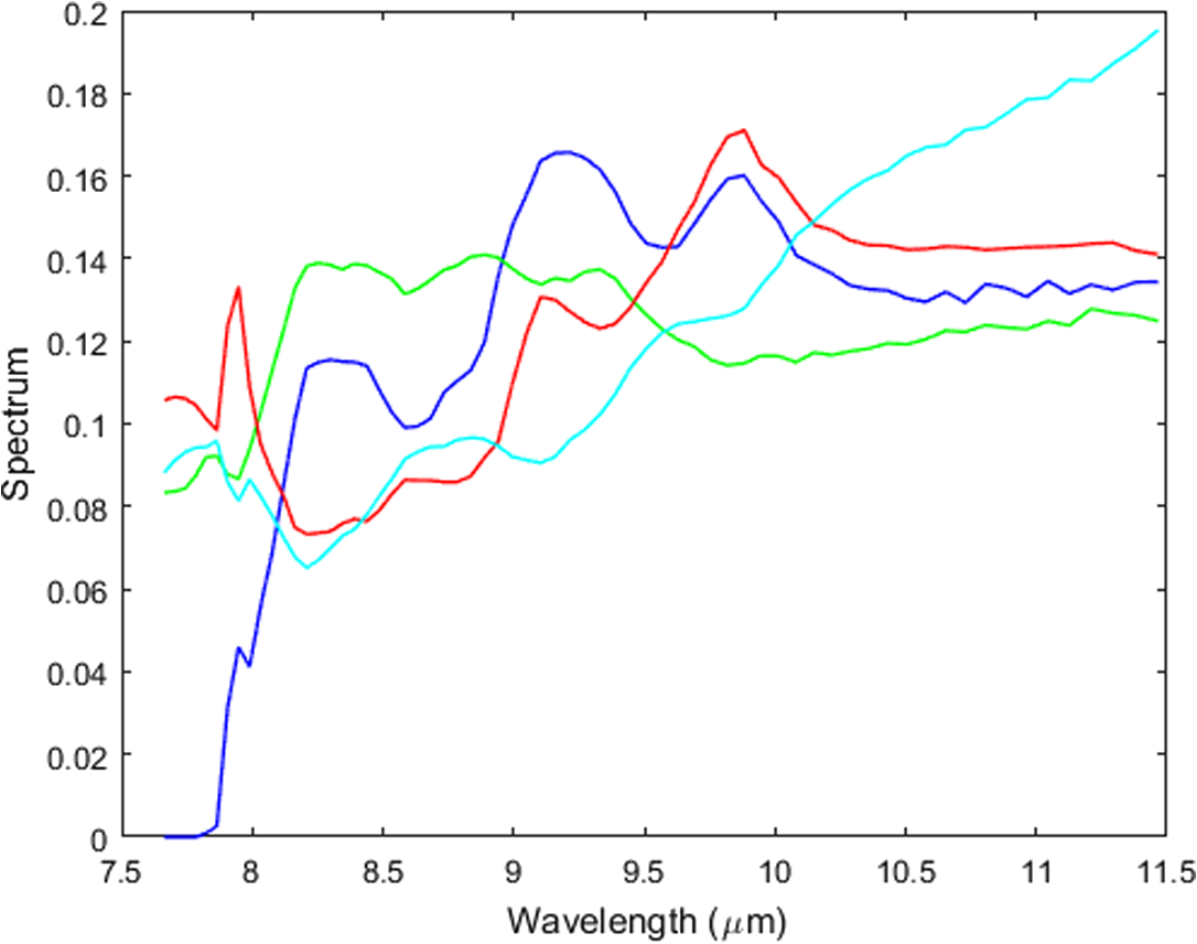
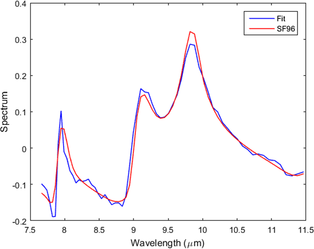
1.

Introduction

Hyperspectral (HS) imaging is a well-established technology having many commercial and military applications. One of those involves using the HS spectral information to detect and locate materials by their known spectral signatures. In general, this is a highly nontrivial task due to the many radiance sources from the clutter background and atmosphere that can easily mask and distort the often weak radiance from the chemical materials of interest. Traditional approaches for separating the radiance components in the data involve either (1) unmixing using the “pure-pixel” or “endmember” assumption that the target materials can be found in a few individual pixels without interference from other radiance sources or (2) the use of likelihood ratio testing in a statistical approach.

The pure pixel or endmember algorithms are more successful on data for which the pure pixel assumption is approximately valid. If such pixels exist and can be identified, least-squares methods can be used to locate the image spatial regions associated with each endmember. Standard simplex-based algorithms, such as N-findr¹ and VCA,² work reasonably well if endmember pixels exist under high SNR conditions.

Targets that are subpixel or mixed pixels are well known to be quite challenging compared to the traditional endmember processing. Those targets are either small or partly concealed by vegetation or other coverings. For this class of targets, statistical methods are used such as the adaptive matched detector³ and the adaptive subspace detector that apply generalized likelihood ratio testing⁴ using background sample covariance matrices to whiten the data followed by subspace projection onto the target spectral subspace.

Both methods make optimistic assumptions about the data—either the existence and detectability of pure pixels—or that the data statistics are well approximated by multivariate normal probability densities. The latter method assumes that the clutter correlation structure can be estimated from the data, assuming spatial homogeneity and the ability to mask the target spectral presence. These are often difficult assumptions to justify in practice.

We have developed an entirely different method for identifying and locating materials on unknown background surfaces using their chemical spectra that makes no prior modeling assumptions about the presence of endmember pixels or the statistics of the surface clutter and sensor noise. Our method also requires no prior knowledge about the background in the absence of the target material. This is the first time that surface detection without dependence on background information, or a priori knowledge of the statistics has been achieved to our knowledge. The generality of our approach makes it potentially applicable to a wide variety of military and civilian scenarios, which are significantly widened by the elimination of the requirement to obtain a clean background data scan. Here, we focus on detecting and discriminating chemicals on background surfaces with arbitrary spectral structure. The method has also been successfully applied to detection of airborne chemicals.

There are three main components to our method: (1) an HS unmixing algorithm⁵ based on the alternating direction method of multipliers (ADMM)⁶ that is used over local subsets of the imaging to resolve the HS data into a set of linearly independent spectral and spatial components; (2) the fitting of those unmixing spectra to a set of candidate template spectra; and (3) a state-of-the-art support vector machine (SVM) classifier for chemical detection, identification, and location.

In Sec. 2, we summarize the ADMM unmixing algorithm without dwelling on the mathematical details. A more complete mathematical summary appears in the Appendix (and in Ref. 5). Although the unmixing is an essential component of our chemical sensing approach, the optical interaction between the chemical reflectance spectral structure and the other radiance components requires an additional material-dependent fitting step to convert the unmixing spectral vectors into estimates of the spectral reflectance of a given material. Section 3 describes the fitting method used for this step. Section 4 describes the SVM developed for detecting and identifying the materials from the spectral fitting step. In Sec. 5, we describe the data collection of reflectance from various amounts of three simulants applied to different background surfaces. Section 6 shows the processing results from these data. Section 7 summarizes the algorithm and its usefulness for surface sensing and other applications, including vapors in the atmosphere.

2.

Alternating Direction Method of Multipliers Hyperspectral Unmixing Algorithm Summary

In this section, we discuss the method we have developed for the unmixing task of resolving HS data cubes into independent components as functions of wavelength band (spectrum) and spatial structure (the analog of abundances). Our discussion is rather informal in that not many mathematical details are given. The Appendix has a more complete mathematical summary, but no derivations. For the latter, the reader is advised to consult Ref. 5.

The motivations for this work were our concern over the ability of standard approaches to provide useful unmixing results for data with no prior information. For example, endmember or pure-pixel algorithms may not work because of the nonexistence of such pixels from spatial resolution or sensor noise limitations. This was already recognized by the likely originator of the term “endmember,” Schowengerdt:⁷ “… endmembers only exist as a conceptual convenience and as idealizations in real images.” Also, the concept of spectrally pure pixels may not have meaning in the LWIR spectral region where our data reside. At the other extreme are unmixing approaches, notably those based on compressive sensing methods, which attempt to fit the data to a sparse set of spectra taken from large libraries. These methods require additional prior information about the data that may not exist in general. Other methods for sparse basis fitting are well known in HS processing. We mention two sources: Dadon et al.⁸ and Adler-Golden and Conforti,⁹ which use sparse fitting but in the context of endmember bases. In contrast, we will show in Sec. 3 that the ADMM unmixing algorithm constructs a sparse basis of spectra directly from the data at each local spatial region.

We formulate the HS unmixing problem in terms of the spectral and spatial arrays $\rho$ and $C$ as the biconvex multiplicative model $G=\rho C+n$, where $G$ represents the HS data cube as $G\in R^{M\times N}$ with $M$ the number of spectral bands (wavelengths) and $N=N_1{N}_2$ is the total number of pixels after stacking the $N_1$ rows and $N_2$ columns into a single vector. We model $\rho \in R_{+}^{M\times L}$ and $C\in R_{+}^{L\times N}$ with $L$ the number of assumed independent components in the cube. $n$ is an additive noise term taken to be zero-mean, independent, and identically distributed with bounded variance.

Because we have only a biconvex optimization problem (convex in either $\rho$ or $C$ given the other, but not jointly convex), we cannot expect to find a global minimizing solution but only approximately optimal solutions that are numerically well-behaved under different initializations of $\rho$. Fortunately, the ADMM formalism can accommodate this biconvex problem and produce good unmixing results by adding appropriate constraints. Its implementation for the unmixing problem leads to an alternating algorithm that, for a given estimate of $\rho$, updates the estimate of $C$ and vice versa until convergence.

Constraints are needed to produce physically meaningful results. They are chosen to be positivity on the spatial and spectral estimates with a unit-vector constraint on the spectrum of each material. The latter replaces the spatially convex constraints used for abundances in the usual endmember approaches and are felt to be more natural physically. The constraints are enforced on the parameter arrays through augmented Lagrangians with Bregman splitting. For the splitting, we have used the splitting orthogonal constraint (SOC) method of Lai and Osher,¹⁰ who introduce auxiliary variables to split the positivity constraints from the estimation of concentration and the spectra. Improved results are often obtained by introducing an $l_1$ regularization of the spectral estimates through total variation (TV), also implemented through Bregman splitting and soft thresholding following Goldstein and Osher.¹¹ The ADMM algorithm in Ref. 5 as well as this paper include this TV regularization.

In addition to the need for constraints, we have observed that much better results are obtained by applying the unmixing and spectral fitting to local subsets of the total data cube. This is particularly true when the materials of interest are present in relatively small regions of the total imagery. The size of the subsets depends on the application. For the chemical-on-surface data with short-range illumination and imaging, blocks of 5 pixels on a side were adequate. For other applications, such as vapor data with larger plume-targets and higher noise levels, blocks of about 30 pixels on a side are more appropriate. These choices allow the processing to adapt to the local structure of the image while supplying enough spatial information to generate good unmixing results. Besides providing better spectral estimates, the use of local processing can be computationally advantageous over a single global fit since the processing steps are identical for each local region and can, therefore, be implemented by parallel processing methods.

3.

Fitting Unmixing Spectra to Chemical Reflectances

In our early experience with the unmixing algorithm, we had hoped that the spectral estimates would prove adequate to identify the radiance components of chemical materials without additional processing. We now know that this is not possible in general. As an example, Fig. 1 plots the unmixing spectra from the ADMM algorithm assuming $L=4$ materials for a $5\times 5\text{pixel}$ block of the Hyper-Cam cube for the simulant SF96 (a silicon oil) as observed on a simulated asphalt road surface. As will be seen below, none of the spectral components in the figure represents the true spectrum of SF96 well, although two of the curves have some resemblance to the actual spectrum. The unmixing spectra are a mixture of the chemical spectrum and the spectral structure of the road surface. Figure 2 plots the SF96 template spectrum labeled as “SF96,” computed as the unpolarized reflectance at normal incidence using the complex refractive index measurements of SF96. The result of the fitting algorithm described below is shown as the curve labeled “fit.” The linear combination of the four unmixing spectra produces a good match to the template.

Fig. 1

Unmixing spectra for SF96 on the simulated road surface.

Fig. 2

Fitted spectrum of SF96 and template model from the road surface data.

With this example as motivation, we show how the unmixing spectra can be used to detect the chemicals. The key is that the unmixing spectra generally do not represent the pure chemicals but contain the reflectances of the chemicals as observed in the background clutter from the surface, illumination source, and possibly the atmosphere. They are, therefore, best regarded as a sparse set of independent basis vectors that can be used to fit the templates of whatever materials may be present. With this interpretation of the unmixing spectra, we are led to the spectral fitting algorithm below.

The basic idea is to model a given chemical reflectance spectrum as a linear combination of the spectral estimates from the unmixing algorithm (after mean subtraction and unit-vector normalization) on each data block. For our purposes, only the spectral shape is important, not the absolute units. The assumptions we make about the spectral fitting in terms of its ability to identify and locate chemical releases are: (1) the template spectrum can be well represented as a linear combination of four to five unmixing spectra when the target material is present in the local subset of the data and (2) the best linear fit to a given template will not fit that template well when the material is not present in the local block. The examples in Sec. 6 support the validity of these assumptions.

We note that the ADMM unmixing algorithm is essential for producing a sparse set of basis vectors that spans the spectral structure of the image sub-block. Although there exists an uncountable infinity of possible basis vectors, the unmixing method used here selects a sparse set that is directly tailored to the image data. Other basis-generating methods, such as principal component analysis, use empirical estimates of the spectral covariance, and the resulting eigenvectors have little relation to the actual spectral structure of the sub-block. This means that many more such vectors would be needed to produce good fits, with a decrease in the discrimination power of the method.

The coefficients in the linear model are estimated by a standard least-squares method, and then the resulting fit is compared to the input reflectance template using an inner product over wavelength-band number. The algorithm pseudocode is given in Algorithm 1. In Algorithm 1, $\rho$ is the $M\times L$ spectral array from the unmixing algorithm, and ${\rho }_M$ is the $1\times M$ row vector representing the unpolarized reflectance of a candidate material after mean-subtraction and unit-vector normalization. The regression estimate of the reflectance is denoted by $\widehat{\rho }$, and $S$ is the inner product of ${\rho }_M$ and $\widehat{\rho }$. Because of the unit-vector normalizations, we always have $|S|\le 1$.

Algorithm 1

Spectral reflectance regression algorithm.

An implicit assumption made above is that the unmixing spectra are linearly independent. We have not experienced dependency problems on the datasets processed thus far for four to five materials. However, for more general applicability to problems requiring a larger number of basis vectors, the spectral unmixing vectors have been orthonormalized within the unmixing algorithm using the SOC method of Ref. 10.

In Sec. 6, the regression fit estimates from various simulant chemicals on different backgrounds will be used as feature vectors to construct SVM classifiers for identifying the materials by the optimization algorithm described next.

4.

Support Vector Machine Classifier

The third component of our chemical sensing approach is a classifier to convert the spectral fitting estimates described in Sec. 3 into decisions for detecting, identifying, and locating the chemical materials on surfaces. We have chosen an SVM classifier for this purpose for several reasons. First, it offers advantages in classification performance on unseen data over earlier methods, such as the Fisher discriminant and neural nets. Second, it directly approximates the theoretically optimal Bayes classifier without needing to estimate conditional probability densities as an intermediate step. Such estimation requires a very large training population to correctly estimate the tails of the density, which are by definition sparse. Using the “kernel trick,” the SVM implicitly maps the feature data (in our case, the spectral fits to a set of candidate templates) into a high-dimensioned space for which hyperplane separation is facilitated. The SVM finds the hyperplane that maximizes the class separation for a given error rate.

The usual training method for an SVM uses quadratic programming (QP) with a combination of equality and inequality constraints. We have found it to be more computationally efficient to recast the usual QP problem into the split Bregman formulation developed by Osher et al.¹² The QP SVM for two classes expressed in the dual Lagrange parameters $\alpha$ becomes

It is convenient to express the constraints on $\alpha$ using the two projection operators:

The QP SVM problem with constraints expressed though projection operators is solved iteratively by the split Bregman method through the recursions in Algorithm 2 with $A=\lambda y{y}^{T}K+I$, $d^0=b^0=0$, ${\alpha }^0=A^{-1}(\lambda 1)$, $k=0$. At convergence, the bias parameter $b_0$ is estimated by the mean difference in the class label vector $y$ and its predicted value $\widehat{y}$ is computed over the training reflectances as follows:

Algorithm 2

SVM classifier training algorithm.

We generalize the binary classifier to more than two classes by the 1-versus-rest method for constructing $J$ binary classifiers, one for each candidate material versus the pooled data from the remaining classes, and an extra null class of junk spectra. The latter class allows the SVM to function as a detector as well as classifier and avoids requiring the decision to always be one of the chemical materials.

For classifier training and initial testing, we selected data from the July 2015 Setup-3 collection performed by Telops on the surfaces Road, Sandy Soil, Cement, and Pebble Soil. More details of these data collections are given in Sec. 5. The inner products $S$ of the simulant templates with the regression fits were used to select as feature vectors fitted spectral estimates having $S\ge 0.9$. For the null class, we selected 254 spectral estimates from the Setup-2 data having no useful radiance signal. Figure 3 plots the selected spectral estimates computed with the regression algorithm described in Sec. 3.

Fig. 3

SVM training data spectra. (a) SF96, (b) DMMP, (c) TEP, and (d) null.

The SVM classifier was trained and tested on alternate samples of these data using a radial basis function kernel width 0.3 and margin parameter 10. The Lagrange parameter in the Bregman training algorithm was set at 10.

For application to new data, we need to construct the appropriate spectral fit $\widehat{\rho }$ since these are our feature vectors. This requires knowledge of the correct template spectrum, which is of course unknown. We, therefore, apply the trained classifier to all material classes within an outer loop over the local sub-blocks of the input HS data. The resulting implementation algorithm is summarized in Algorithm 3. The required inputs are $\rho$, the spectral components from the unmixing algorithm; ${\rho }_r$, the set of training spectral fits as a function of wavelength and training sample number; the SVM arrays from the training, $\alpha$, $Y_r$, $b$; and ${\rho }_M$, the set of reflectance templates as a function of wavelength and class. The outputs from the algorithm are the decision function images $f$ for each sub-block and class, and fitted spectra $\widehat{\rho }$ as functions of wavelength, sub-block indices, and class. Section 6 will show the application of this classifier to chemicals on different surfaces.

Algorithm 3

SVM classifier implementation algorithm.

In Algorithm 3, $F$ is the spectral fitting algorithm in Algorithm 1, and $K$ is the radial basis function kernel of the SVM classifier. The parameters $N_{\text{block}}$ and $J$ are the number of sub-blocks in the HS data cube and the number of chemical classes (currently 4).

5.

Collection of Reflectance Data for Contaminated Surface Detection

Data to support algorithm development were collected with components that could be used in an eventual surface detection sensor, arranged to operate at close range, such as handheld or from the underside of a military vehicle, and with target surfaces and chemicals that simulated real-world types as closely as possible. It was found in previous studies that the use of simulated data or data from too idealized conditions could misdirect development. The data were obtained in four separate test events during the course of the 2014 to 2016 program, including outside under sunlight, and inside a building under ambient fluorescent lighting.

A schematic of the final data acquisition system is shown in Fig. 4. It is composed of a linear glowbar with condensing elliptical mirror illuminator and an unpolarized HS camera receiver placed in the specular reflection condition to maximize the signal. It was found in separate measurements that even for the relatively rough test surfaces, reflection occurred with a pronounced intensity lobe in the specular direction. The minimum incidence and reflection angles of 21 deg were determined by the size of the components. Range of the illuminator to the target was 46 cm and range from target to camera was 150 cm, determined by the camera optics. The elliptical mirror was found necessary to improve radiance on the target compared to the commercial reflector supplied with the glowbar, which was made available for the final field test. The data analysis below relates to this final data acquisition event.

Fig. 4

Data collection setup.

A schematic of the elliptical mirror and glowbar arrangement is shown in Fig. 5. The glowbar had a diameter of 7.6 mm and heated length of 23 cm. It was located 2 cm from the mirror surface at one ellipse focus. For an input power of 350 W, the measured temperature at the rod center was 730°C. Cooling fins and a fan attached to the backside of the mirror (not shown in the figure) maintained the mirror at 28°C. In practice, the mirror temperature could be allowed to rise, thereby further increasing intensity on the target. The mirror was configured for an ellipse interfocus distance of 46 cm such that radiation from the glowbar would be concentrated onto the target located at the second focal point. Spatial scans with an irised detector showed a stripe radiation pattern at the target location with full width at half maximum of $\sim 7\mathrm{cm}$ transverse to the heated rod long dimension and a roughly 5% variation in intensity over the central 6 cm of the target parallel to the rod. The full width half maximum in the parallel direction was about 9 cm. Measurements showed that intensity on target with the elliptical mirror was increased by roughly a factor of 8 over that with the commercial reflector and a factor of 21 compared to a bare heated glowbar without reflector.

Fig. 5

Elliptical mirror and heated rod schematic.

The HS camera receiver was provided by Telops, Inc., their field-portable Hyper-Cam-LW.¹³ The Hyper-Cam sensor uses a Michelson-type interferometer to spectrally modulate the IR radiation from the scene, thereby allowing for demodulation of the acquired interferograms to produce raw spectra using the Fourier transform. The detector module for generation of IR images consists of a cryo-engine-cooled, HgCdTe focal-plane array of $320\times 256\text{pixels}$ sensitive over the 8- to $11\text{-}\mu \mathrm{m}$ long wavelength band. The data acquired as raw spectra are stored as datacubes, three-dimensional arrays of values used to describe a series of images. Successive images in the datacube represent either interferogram data at different optical path difference fringe numbers or spectral data at different wave numbers. The entire datacube is acquired during a single scan, in either the forward or the reverse direction of the interferometer inside the sensor. The Hyper-Cam sensor is software controlled and uses an Ethernet communication link. Datacubes from the Hyper-Cam sensor are sent to a frame-grabber card in the interface computer. Calibration of the camera can be carried out periodically by rotating in front of the objective lens, a blackbody with temperature set over the range 10°C to 60°C.

The camera can operate with a spectral resolution of 0.25 to $150{\mathrm{cm}}^{-1}$. In order to achieve the desired tradeoff in spectral accuracy, signal strength, and scan time, a resolution of $8{\mathrm{cm}}^{-1}$ and $140\text{-}\mu \mathrm{s}$ integration time were used for the data captures described below. The nominal camera single pixel projection on the target was $\sim 0.2\mathrm{mm}$, providing for good resolution of the several mm-size chemical droplets.

The commercial style Hyper-Cam-LW is approximately $40\times 30\times 8{\mathrm{cm}}^3$ in size and weighs 29 kg. Telops, Inc. has produced a reduced size, $23\times 17\times 10{\mathrm{cm}}^3$ model for airborne applications. In the case of an imaging spectrometer (for high speed data capture), where the moving mirror interferometer would be replaced by a fixed wavelength dispersing prism for single pixel line scanning in a push broom pattern, the size and weight could be reduced further.

Photographs of the target surfaces are shown in Fig. 6 and include cement aggregate, in which cement plaster was mixed with small stones, and asphalt aggregate, in which stones were mixed with asphaltum. A range of stone sizes made up the aggregate with the larger stones having a scale size of about 1 cm. Single droplets of the three simulant test chemicals can be seen wetting the cement surface, but the spots on the asphalt are not readily visible. During testing, the single-target surfaces with a specific number of drops added to the wetted positions were placed in position below the elliptical mirror illuminator.

Fig. 6

Target surfaces, asphalt, and cement aggregate.

The test chemicals were SF96, triethyl phosphate (TEP), and dimethyl methylphosphonate (DMMP). The SF96 was manufactured with a viscosity of 1000 cSt. TEP and DMMP were obtained with viscosities of 10 cSt and subsequently thickened to $\sim 1000\mathrm{cSt}$ by mixing with small amounts of the long chain polymer K-125 produced by Dow Chemical. Measurements of the real and complex indices of refraction showed that thickening did not alter them.

Data acquisition was made simultaneously for the three test chemicals deposited on each surface. Tests included an increasing number of deposited droplets placed in a single position. The targets were removed from underneath the illuminator between acquisitions to prevent heating from the intense beam. In a final test, a mixture of all three chemicals was placed at each position to provide a more complicated target that could be interpreted as a single target chemical with interferents.

6.

Algorithm Testing on Surface Contamination Data

As discussed in Sec. 5, there were four data collection efforts under the project. For simplicity, we concentrate on data collected from the fourth test in May 2016 (although the SVM classifier was trained on data from the third collection.)

The three thickened simulant materials SF96, DMMP, and TEP were used; the background surfaces were simulated asphalt road and cement aggregate; and the chemical concentrations were incrementally increased from one drop (0.03 g), to three, six, and nine drops of each material with an extra collection at the conclusion of the test that added three drops each of the other materials to the nine drops of already deposited chemical. About 15 or 30 min delays were used between the successive deposits to allow the chemical spots to diffuse on the surfaces. The increasing amounts of material were to be used to estimate the minimum detectable concentration of each material. HS data from these surfaces were processed using the algorithms described above.

We show the decision function images from the processing of the Test #4 data. As above, the processing steps were: (1) unmixing the data for four materials (five materials for the Cement_Mix data) in contiguous blocks of 25 pixels each; (2) spectral fitting of each set of four to five spectra from the unmixing to each of the template spectra; and (3) passing each spectral fit into the SVM classifier trained for the three simulant materials and the null class spectra.

Figure 7 plots the decision function images for the file Road_01 that represents a single drop of each simulant on the simulated road surface. We see clear evidence of the three simulants with little indication of the materials not present. Figure 8 compares the template spectra with the spectral fits at the image sub-blocks having the peak decision function values. The peak correlation coefficients for the three materials were 0.9805, 0.9637, and 0.9871 for SF96, DMMP, and TEP, respectively. The time to perform the unmixing (the slowest part of the algorithm) was 2.75 s for the total image area shown. We see that fits using only four unmixing components are able to fit the templates quite well.

Fig. 7

SVM decision function images for the Road_01 dataset. (a) SF96, (b) DMMP, and (c) TEP.

Fig. 8

Comparison of templates and the best fits for the Road_01 data. (a) SF96, (b) DMMP, and (c) TEP.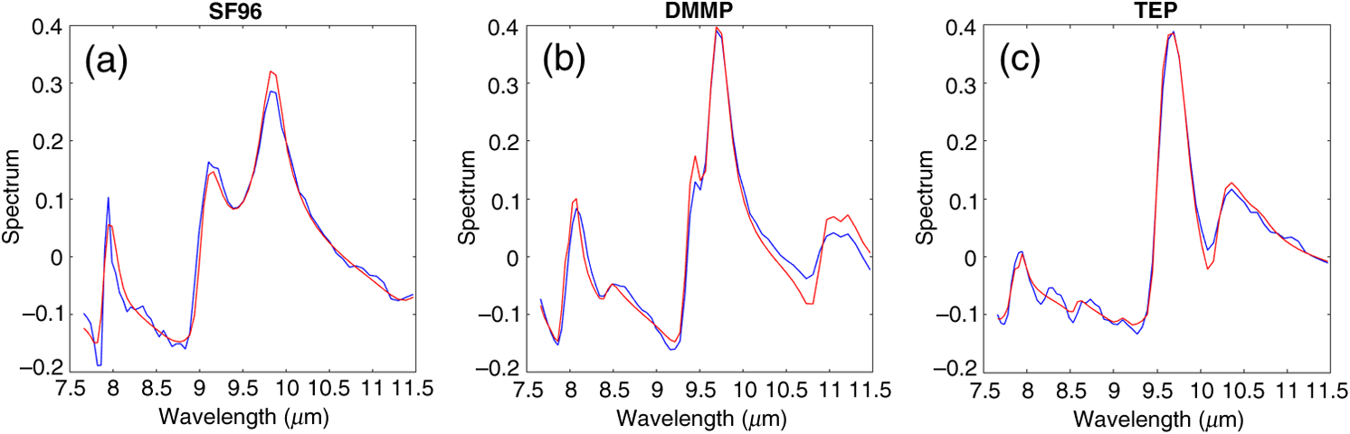

Figure 9 plots the decision functions for the Cement_01 data for 1 drop each of the simulants on the cement aggregate surface. We again observe all three materials but with a weaker indication of SF96 compared to DMMP and TEP.

Fig. 9

SVM decision function images for the Cement_01 dataset. (a) SF96, (b) DMMP, and (c) TEP.

As the last surface sensing application, Fig. 10 shows the SVM decision functions for the Cement_Mix data with nine drops of each simulant at each of the three locations of the initial one-drop disseminations. These data were collected on the cement surface and processed using five materials in the ADMM unmixing step. The spatial sub-blocks were again taken to be 25-pixel squares. All three materials are evident at each dissemination region. The best fit spectra for each material are shown in Fig. 11. The processing was able to find the materials within spots having multiple chemicals at the same spatial locations.

Fig. 10

SVM decision function images for the Cement_Mix dataset. (a) SF96, (b) DMMP, and (c) TEP.

Fig. 11

Comparison of templates and the best fits for the Cement_Mix data. (a) SF96, (b) DMMP, and (c) TEP.

7.

Summary and Conclusions

We have described and illustrated a new method for using HS imaging data to detect, identify, and locate chemical materials on arbitrary spectral backgrounds by fitting the set of spectral estimates from an unmixing algorithm to a set of candidate chemical spectra. The unmixing and spectral fitting are done locally over nonoverlapping blocks of pixels. The ADMM HS unmixing algorithm, summarized here and presented in more detail in Ref. 5, does not assume the presence of endmember pixels and does not require background data subtraction, or modeling assumptions, such as the validity of multivariate normal statistics.

With reference to the latter class of processing techniques, the optimal (likelihood ratio) processor would attempt to estimate the spatial covariance of the scene, and spatially whiten the target and background combination prior to matched filtering with the chemical spectral templates. We would not claim that our HS detection algorithm will perform better than the likelihood ratio processor on data for which likelihood processing is best suited, i.e., spatially homogeneous multivariate normal data with good covariance and clean background estimates. The question is, how often will such data be available? We believe that the main advantage of our approach is that it can produce good results on data for which these assumptions are not well-satisfied.

Most of the processing time in our approach is taken by the unmixing and fitting/classification steps (in the case of a large library of candidate materials). Both of those steps perform the same operations on all pixel blocks and library materials, and are, therefore, parallelizable and could be done in real time. Also, the chemical templates could be provided with absolute scales making the detection results interpretable in concentration units.

The regression algorithm that fits the candidate spectral templates to the unmixing spectra is the reverse of most HS algorithms that fit the data to selected spectral samples from large libraries. In our approach, the roles of the target function and independent fitting functions are reversed. Our basis functions are a sparse set produced locally from the data via the unmixing algorithm, and the target functions are the set of candidate materials. The latter set can be quite large, but the simple regression fitting proposed here is very fast, and likely to be more efficient than the compressive sensing algorithms with their large spectral libraries, currently in vogue.

The processing requirements needed to apply the proposed chemical sensing algorithm to the contaminated surface and other HS data applications are (1) a good unmixing algorithm and (2) a set of hypothesized target spectral templates. The assumptions in terms of the spectral fitting are that (1) the template spectrum can be represented well as a linear combination of a small number of the locally estimated unmixing spectra when that material is present in the data and (2) conversely, the best linear fit to a given template will not match the template well when that material is not present. We have empirically verified those assumptions on a wide variety of processing cases.

Finally, we have shown that data from training sets collected on a representative population of target material depositions can be used to train a classifier such as the SVM. We used the SVM because of long-time familiarity, but other kernel-based large margin classifiers, such as the radial-basis-function network, could work as well. The main thing is to use a modern classifier trained on lots of data. We have successfully implemented the SVM for chemical contamination sensing on spectrally unknown surfaces. Detection of chemicals on roads could be achieved in real time from a moving vehicle by using the highly accurate and computationally efficient algorithm, the high incident intensities from an emitter with elliptical mirror concentrator, and an imaging spectrometer receiver with fixed prism dispersion. Note that the method described here does not require collection of data for the two polarization states, which would otherwise complicate the sensor and significantly impair the detection timeline.

Our choices of the number of unmixing spectra (four to five) and the pixel block size (25 pixels) were made to match our data. For more complicated backgrounds under lower SNR conditions, both would need to be larger. For example, experience with vapor sensing in the atmosphere against natural LWIR clutter backgrounds suggests that six to eight unmixing components with block sizes on the order of 30 pixels on a side are more appropriate. Indeed, we have achieved good results on vapor release data collected at Dugway Proving Ground, Utah, against natural thermal backgrounds with a Hyper-Cam sensor¹⁴ using a very similar approach to the first two components of the algorithm presented here. That work will be described in a future paper.

Other applications include airborne HS data collection for natural resource and military sensing. In the event that detection at longer ranges is required, higher power illuminators in the form of wavelength agile, long wavelength lasers could be considered. Broadband Quantum Cascade and ${\mathrm{CO}}_2$ lasers would be possible candidates, too.