Extracting distribution and expansion of rubber plantations from Landsat imagery using the C5.0 decision tree method

Zhongchang Sun; Patrick Leinenkugel; Huadong Guo; Chong Huang; Claudia Kuenzer

doi:10.1117/1.JRS.11.026011

2 May 2017 Extracting distribution and expansion of rubber plantations from Landsat imagery using the C5.0 decision tree method

Zhongchang Sun, Patrick Leinenkugel, Huadong Guo, Chong Huang, Claudia Kuenzer

Author Affiliations +

Journal of Applied Remote Sensing, Vol. 11, Issue 2, 026011 (May 2017). https://doi.org/10.1117/1.JRS.11.026011

Abstract

Natural tropical rainforests in China’s Xishuangbanna region have undergone dramatic conversion to rubber plantations in recent decades, resulting in altering the region’s environment and ecological systems. Therefore, it is of great importance for local environmental and ecological protection agencies to research the distribution and expansion of rubber plantations. The objective of this paper is to monitor dynamic changes of rubber plantations in China’s Xishuangbanna region based on multitemporal Landsat images (acquired in 1989, 2000, and 2013) using a C5.0-based decision-tree method. A practical and semiautomatic data processing procedure for mapping rubber plantations was proposed. Especially, haze removal and deshadowing were proposed to perform atmospheric and topographic correction and reduce the effects of haze, shadow, and terrain. Our results showed that the atmospheric and topographic correction could improve the extraction accuracy of rubber plantations, especially in mountainous areas. The overall classification accuracies were 84.2%, 83.9%, and 86.5% for the Landsat images acquired in 1989, 2000, and 2013, respectively. This study also found that the Landsat-8 images could provide significant improvement in the ability to identify rubber plantations. The extracted maps showed the selected study area underwent rapid conversion of natural and seminatural forest to a rubber plantations from 1989 to 2013. The rubber plantation area increased from 2.8% in 1989 to 17.8% in 2013, while the forest/woodland area decreased from 75.6% in 1989 to 44.8% in 2013. The proposed data processing procedure is a promising approach to mapping the spatial distribution and temporal dynamics of rubber plantations on a regional scale.

1. Introduction

As a result of the increasing global demand for natural rubber products, rubber plantations have become very lucrative and have thus been expanding drastically in many regions over the last several decades.¹^,² Asia, in particular, has become the world center of rubber production, accounting for 92% of the global natural rubber supply.³ Over the last few decades, more than one million hectares of land have been converted to rubber plantations in nontraditionally rubber growing areas of China, Indonesia, Thailand, Vietnam, Malaysia, and India.⁴^,⁵

The conversion of natural and seminatural forests and even croplands to rubber plantations has become a significant land cover (LC) and land use change process in the past decade.⁶ On one hand, this transformation has a positive influence on agricultural systems by providing increased profits and improving farmers’ financial stability.²^,⁷ On the other hand, however, it can have significant adverse ecological impacts on water balance, hydrological systems, carbon budgets, habitats, and biodiversity.⁴^,⁸^–¹¹ Rubber plants are often referred to as small “water pumps” since they destroy the water-conservation services of natural forests and hasten soil-erosion processes.⁸^,¹² In some reported cases, streams have dried and villages have lost their water supply.¹³ Furthermore, the use of fertilizer and pesticide to stimulate rubber plants’ growth leads to water-body pollution and threatens the survival of many aquatic animals and plants. In terms of some aims of reducing emissions from deforestation and forest degradation, carbon sequestration of rubber plantations is limited in comparison to that of natural forests, which means that expansion of rubber plantations very likely results in significant increase in net emission of carbon dioxide.¹⁴^,¹⁵ In the case of the Xishuangbanna region, China, the large-scale conversion of forests to rubber plantations has likely played an important role in changes of local climate, such as diminishing rainfall, increasing the likelihood of more severe droughts, and drastically lowering the frequency of fog between the mid-1950s and the mid-1980s.⁸^,¹² Therefore, it is of great importance for local environmental and ecological protection agencies to research the distribution and spread of rubber plantations and to be able to monitor their dynamic changes.

In view of these developments, the accurate, high-resolution mapping and monitoring of the expansion of rubber plantations is necessary. A number of studies have been conducted to this end. Shigematsu et al.¹⁶ employed data from rubber wood processing and retailing companies to estimate the production of rubber wood from 1996 to 2011 in Cambodia. However, such statistical methods do not capture the spatial distribution of rubber plantations. In addition, these data and statistics in many cases are often insufficient or even unavailable, especially in developing countries, and can be politically biased. Due to their low cost, wide coverage, short cycle, and suitability for large area mapping, satellite images have been widely applied for the identification and delineation of rubber plantations. The current studies, which are related to the extraction of rubber plantations from remote sensing imagery, can be categorized into three broad groups. The first group focuses on the use of spectral signatures together with cluster analysis and traditional classifiers to identify and map rubber plantations. Li et al.¹⁷^,¹⁸ used six periods of Landsat MSS/TM/ETM+ images acquired between 1976 and 2007, together with a 1:50 000 digital elevation model (DEM), to analyze how patterns of land use, cover type change, and transfer rates between cover types were affected by topography in Xishuangbanna. The relationship between rubber growth and topography was also investigated. Zhang et al.¹⁹ used georeferenced field data and Landsat TM images from May to August of 2008 to conduct a maximum likelihood supervised classification that produced an area of $4.1676 \times 10^{5} {ha}^{2}$ for rubber plantations in Hainan Island, China. Chen et al.,²⁰ and Li et al.²¹ used HJ-1 satellite data and field sampling data to estimate the distribution of rubber trees based on a decision-tree (DT) classification in the Xishuangbanna area in 2011. Li and Fox¹^,⁵^,²² integrated the Mahalanobis typicality with a multilayer perceptron (MLP) neural network to identify rubber trees in mainland southeast Asia using spectral data from MODIS and ASTER together with Landsat imagery. Their method greatly reduced the commission errors for mature and young rubber plantations, and was able to successfully overcome the earlier overestimation problem. Chen et al.²³ mapped rubber plantations in and outside protected areas and their net present value for the years 1988, 2002, and 2010 from Landsat and RapidEye data. The second group of studies relies on the temporal signals of optical images to delineate rubber trees. Tan et al.²⁴ applied normalized difference vegetation index (NDVI) time-series data from MODIS and China’s Feng-Yun-3A (FY-3A) satellite to represent the phenological signatures of rubber plantations, and then used the intra-annual temporal profiles of this class to delineate plantations in Hainan, China. Liu et al.²⁵ proposed a new method to identify and map rubber plantations based on phenological characteristics of vegetation cover type. Using this method, an accuracy of 76.42% was achieved for young rubber forests ( $< 10$ years old) and 92.50% for mature rubber forests ( $> 10$ years old) in Xishuangbanna in 2010. Senf et al.⁶ tested a new approach for mapping rubber plantations and natural forests with the random forest classification algorithm using phenological metrics derived from MODIS enhanced vegetation index (EVI) and short-wave infrared (SWIR) reflectance time series in the Xishuangbanna area. Fan et al.²⁶ presented a phenology-based vegetation index differencing method for rapidly mapping rubber plantations using Landsat operational land imager (OLI) data. Li et al.²⁷ used a simple and effective phenology-based algorithm for detecting and mapping rubber tree plantations through vegetation indices by combing a Landsat-derived vegetation map and a DEM mask in Xishuangbanna. The third group concentrates on accurately mapping the fractional extent of rubber plantations by combining synthetic aperture radar (SAR)-derived forest maps with phenology derived from optical images. In contrast to optical sensors, SAR can penetrate clouds and has advantages in mapping tropical forests, particularly at longer wavelengths (e.g., L-band SAR) that are capable of penetrating tree canopies. Dong et al.²⁸ mapped three forest types, including rubber plantations, on Hainan Island using advanced land observing interferometric synthetic aperture radar (ALOS PALSAR), MODIS NDVI, MODIS EVI, and land surface water index time series. Dong et al.² provided an insight into the potential of integrating cloud-free 50-m PALSAR and multitemporal Landsat imagery for mapping deciduous rubber plantations in moist tropical regions. Kou et al.²⁹ presented a simple method for mapping rubber plantation areas and their stand ages by integration of PALSAR 50-m mosaic images and multitemporal Landsat TM/ETM+ images. Chen et al.³⁰ explored the potential utility of integrating 25-m cloud-free phased array type L-band synthetic aperture radar (PALSAR) mosaic product and multitemporal Landsat images to map forests and rubber plantations in Hainan Island, China.

A number of challenges with respect to the mapping of rubber plantations using remote sensing techniques are summarized here.¹^,²^,⁵ First, frequent cloud cover in the focal region of southeast Asia has a significant effect on rubber plantation delineation, especially for optical imagery. Second, mature rubber trees have multispectral reflectance characteristics similar to those of tropical evergreen vegetation; thus, misclassifying second-growth forests as rubber trees poses a major obstacle to accurate classification and results in overestimates of rubber growth. Third, young rubber trees are grown in a complex and heterogeneous mix of land-cover types, including bare or fallow soil and mixed scrub, and/or are intercropped with rapidly growing cash crops, such as cassava and pineapple. Even after 3 to 4 years of growth, rubber tree canopies cover only a small fraction of the total planted area in which they are grown. Image pixels identified as containing young rubber trees are often confused with other, more dominant, LC types. Finally, high intraclass variability between rubber trees of different ages poses another difficulty for discriminating rubber trees from other LC types.

At present, various advanced approaches based on the studies described above have been developed to extract rubber plantations from satellite images and also to quantify them. These approaches mainly include: (1) maximum likelihood supervised classification;¹⁹ (2) support vector machine (SVM);³¹ (3) random forests;⁶ (4) artificial neural networks;¹^,²⁸ (5) DT;²¹^,²⁹^,³⁰ and (6) the object-oriented classification method.²⁵ Although many neural network models have been developed, the MLP neural network (MLPNN) is the most widely used.¹ However, the MLPNN has some limitations,³² including: (1) it is sensitive to the network structure, (2) it suffers from the local minima problem, and (3) the training process for the MLPNN algorithm is not consistent. For the SVM, the major difficulties are parameter optimization and lack of model interpretability.³² In this paper, a robust algorithm, a boosted DT named See5/C5.0, is used for extracting the expansion of rubber plantations.³³ In contrast to other algorithms, the C5.0 method incorporates new methods in machine learning, such as adaptive boosting, an ensemble method that has been widely used to enhance classification accuracy and to minimize sensitivity to noises.³⁴^,³⁵

The main objective of this research is to derive the dynamic changes in rubber plantations that have occurred within the autonomous prefecture of Xishuangbanna, China, over a time span of more than two decades from Landsat TM imagery using a C5.0 DT classification method. Although much work on rubber plantation mapping based on satellite imagery has been performed already, this paper includes findings and answers related to some pressing questions that have not been addressed in previous studies.

1. How did the distribution of rubber plantations change between the late 1980s and the present? Li et al.¹⁷^,¹⁸ and Chen et al.²³ have already detected changes that occurred in Xishuangbanna between 1976 and 2010. However, rubber development in southeast Asia began to intensify only at the end of the 1980s.¹² Therefore, the observation period chosen for this study (1989 to 2013) is the period covering the most intense period of rubber development in this region. The choice of this period thereby close knowledge gaps and provides the research community with an up-to-date depiction of the distribution of rubber plantations within more than 92% of the autonomous prefecture Xishuangbanna.
2. About 95% of Xishuangbanna is covered by mountains and hills. This has a big effect on the classification results. Although some studies on the detection of rubber plantations have included topographic and atmospheric correction of satellite images, haze and shadow removal has not been conducted.²^,¹⁸^,²²^,³⁶ In this study, in order to reduce the effects of haze and the terrain, an atmospheric and topographic correction of the satellite data, including haze removal and deshadowing, is performed using the Atmospheric/Topographic Correction for Mountainous Terrain (ATCOR3) software developed by DLR (German Aerospace Center).³⁷ The ATCOR3 combining with classification method was widely used to improve classification accuracy of LC, especially in mountainous areas.³⁸^–⁴¹ This correction is implemented as part of a reasonable, practical, and semiautomatic data processing procedure for the mapping of the rubber plantation distribution.
3. A third feature in this paper is to explore the potential of the new Landsat-8 OLI sensor for the identification and quantification of rubber plantations. Furthermore, the suitability of the new Landsat sensor for the mapping of rubber plantations was evaluated by comparing with TM/ETM+ images.

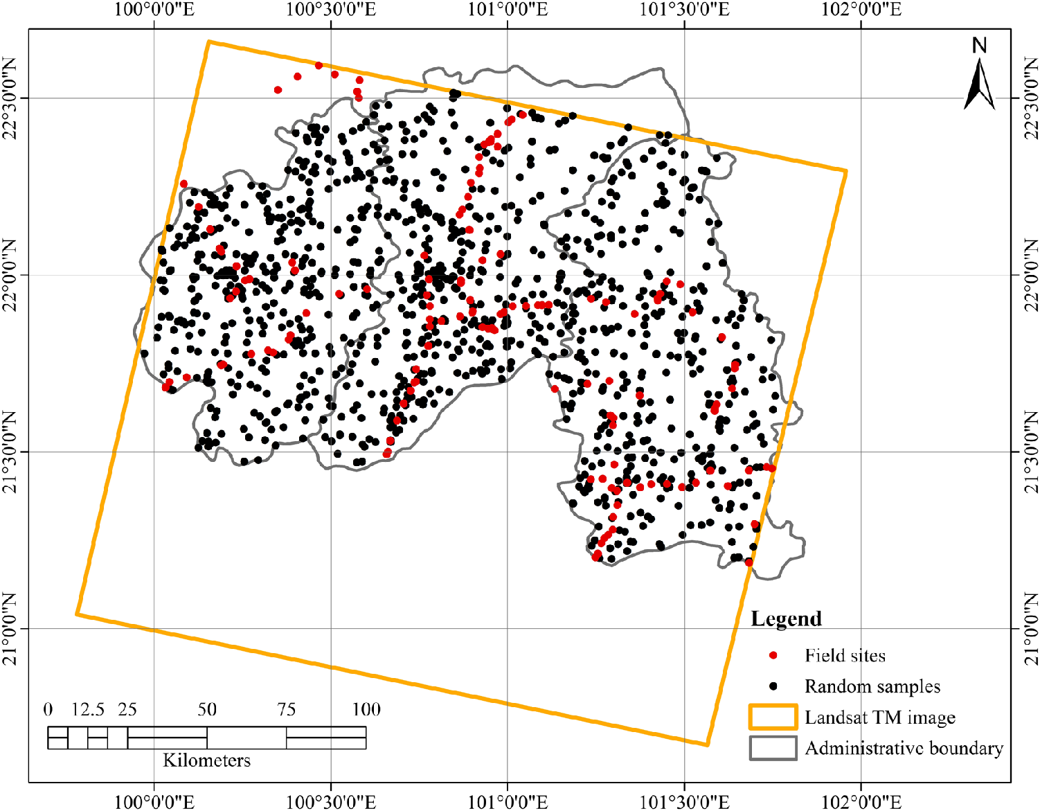
The rest of this paper is organized as follows. Section 2 describes the study area and the datasets used, Sec. 3 introduces the methodology, Sec. 4 presents the results and analysis, Sec. 5 contains the discussion of the results; and Sec. 6 presents the conclusions.

2. Study Area and Datasets

2.1.

Study Area

The autonomous prefecture of Xishuangbanna in Yunnan Province, China, is located in the southwest of the country, covering an area of $19,120 {km}^{2}$ with a population of around 1.13 million in 2010 (Fig. 1). Xishuangbanna is subdivided into three counties (Jinghong, Menghai, and Mengla), and borders Laos to the south and Myanmar to the southwest. The Mekong River (named the Lancang River within the territory of China) flows through central Xishuangbanna, comprising more than 20 important tributaries along this river; consequently, the region contains many river valleys and small basins. About 95% of the prefecture is a mountainous area with its elevation ranging from 460 to 2415 m above sea level. Xishuangbanna is the only region in continental China that has a tropical, monsoon-influenced climate, resulting in a wet season from May to October and a dry season from November to April.²⁵ The average temperature ranges from 19.7°C to 22.9°C and the annual precipitation varies between 1036.1 and 2431.5 mm.

Fig. 1

The study area.

Although Xishuangbanna comprises just 0.2% of the nation’s landmass, it contains 25% of its higher plant species, 36% of its birds, and 22% of its mammals.¹³ Forests in Xishuangbanna can be differentiated into four primary forest types: tropical rain forest, tropical seasonal moist forest, tropical mountain evergreen broad-leaved forest, and tropical monsoon forest. Although the rubber trees shed their leaves for 2 or 4 weeks during the coldest and driest months (January to March),⁸ the climate in this region is suitable for rubber trees and they grow faster here than in many other regions in southeast Asia. Xishuangbanna is China’s second-largest natural rubber production base. Rubber was first introduced to Xishuangbanna in the early 1950s.⁴² In the early 1980s, rubber plantations were established within state farms. After the 1990s and especially in the past decade, rubber plantations have expanded rapidly in Xishuangbanna along with the increased price of rubber. Before the 1990s, rubber replaced large expanses of tropical rain forest at elevations below 800 m.⁸ The expansion of rubber plantations, however, soon shifted to include areas at higher elevations as well. In recent years, the upper limit of rubber plantations has increased continuously from 1000 to 1400 m.¹⁸

2.2.

Datasets

The temporal patterns of rubber distribution were derived from two Landsat TM images (January 11, 1989 and January 27, 1989), a Landsat ETM image (March 14, 2000) and a Landsat-8 OLI image (June 14, 2013). In our study area, most vegetation, including mature rubber plantations, are evergreen species. Although a young rubber plantation is defoliated in dry seasons, its distribution in the study area is limited.²⁵ Therefore, the images were selected without considering the phenology characteristics of rubber plantations. These Landsat images (with path130/row45) cover more than 92% of the whole autonomous prefecture Xishuangbanna. These standard level-one Landsat image products were obtained from the United States Geological Survey Earth Resources Observation and Science Data Center. Two Landsat TM images in 1989 were used to generate the 1989 rubber distribution, with information from January 11 used to fill in cloud-covered areas in the January 27 image. These images were rectified to a Universal Transverse Mercator coordinate system with a pixel size of 30 m. All nonpanchromatic channels of the ETM and OLI-thermal infrared sensor (TIRS) images and all channels of the TM image were used in the classification. The Landsat-8 satellite was successfully launched on February 1, 2013, and carried two main loads: the OLI and the TIRS. The OLI instrument images the Earth in nine spectral bands covering the visible, near-infrared and SWIR portions of the electromagnetic spectrum. All bands are acquired at 12-bit radiometric resolution; eight bands have a spatial resolution 30 m while one, the panchromatic band, has a resolution of 15 m.

We conducted field surveys of rubber plantations and other LC types in 2010. Using a handheld global position system device, 152 georeferenced field sites in the study area were collected for training and validation of the classification results. The locations of these ground truth samples are shown in Fig. 1.

3. Methodology

Figure 2 shows an overview of the data processing procedure. The flow chart is composed of four parts, including data preprocessing, C5.0 classifier “ruleset” construction, classification/accuracy assessment, and LC change analysis. In LC change analysis step, multitemporal change analysis was based on a pixel-to-pixel postclassification using ArcGIS software. A detailed description of the atmospheric and topographic correction, the classification using the C5.0 algorithm, and the accuracy validation is given in the following sections.

Fig. 2

Flow chart of the classification procedure. The darker gray boxes represent datasets inputs and products generated in this context; the light gray boxes represent automatic computational processes; and the dark gray boxes represent manual processes.

3.1.

Atmospheric and Topographic Correction

In order to reduce effects due to haze and the terrain, the ATCOR3 software developed by DLR was performed.³⁷ In addition, Shuttle Radar Topography Mission (SRTM) DEM data with a spatial resolution of 90 m were used as the ATCOR3 parameter for atmospheric and topographic correction. Therefore, the DEM was resampled to 30 m to match the pixel size of the Landsat images. The complete sequence of processing for sensors with water vapor bands and a SWIR band (1.6- or $2.2 - μ m$ region) consists of the following steps:³⁷ (1) masking of haze, cloud, water, and clear pixels; (2) haze removal or cirrus removal; (3) deshadowing based on the matched filter approach; (4) masking of reference pixels; (5) calculation of visibility, visibility index, and aerosol optical thickness for reference pixels using DEM data; (6) (if required) updating the path radiance in the blue-to-red spectral region providing a blue spectral band exists; (7) water vapor retrieval using the previously calculated visibility map based on terrain elevation; (8) reflectance spectrum retrieval using a pixel-based water vapor and visibility map; and (9) temperature/emissivity retrieval using DEM information if thermal bands exist.

In the specific data processing procedure, the calibration file was first generated based on the Landsat metadata file. In case of the rugged terrain, some input files including image file, calibration file, as well as DEM file were specified for ATCOR3. DEM is used to calculate slope/aspect images, the sky-view factor, and topographic shadow. The pixel size of the DEM data must be the same as the image pixel size for ATCOR3 software. According to different Landsat data, different sensors and bands were selected. Since our study area belongs to a tropical atmosphere, the aerosol was set to rural. The date of image, the solar zenith, and pixel size were obtained from satellite header. The parameters of the adjacency range were set to default value 1 km. According to DEM data, the average ground elevation was set to 1.06 km by ATCOR3 software. ATCOR3 uses the dark dense vegetation approach to calculate the best visibility for an image. The parameters of visibility were set to 23 and 46 km corresponding to Landsat TM/ETM+ and Landsat 8 image, respectively. In image processing, haze and shadow removal were performed, and the parameters of haze and shadow removal were set to fault values.

3.2.

C5.0 Rulesets Classifier

Training samples were collected based on cross-validating the Landsat images with high resolution Google Earth images and the georeferenced field sites in the study area. The target variables consisted of six LC classes: urban, rubber plantations, forest/woodlands, shrubs/other vegetation, nonvegetated land, and water bodies. A group of polygon regions of interest (RoIs) for each LC class was manually drawn based on the Landsat images, Google Earth imagery, and field sites; these polygon RoIs were later divided into training and testing samples (shown in Table 1). Then, these polygon RoIs were converted to KML files. We further selected and checked samples’ quality by cross-validating of the samples, Google Earth image, Landsat images, as well as georeferenced field sites. As Google Earth imagery within the study area was available for the time period 1999 to 2014 only and the Landsat images (especially for the images acquired in 1989) were out of data in the study area, the polygon RoIs for 1989 were predominantly selected by cross-comparison with the 2013 Landsat image. Only areas that had not changed between 1989 and 2013 were selected by visual interpretation. In addition, the size of the polygon RoIs for each LC class was also considered and should be approximately the same during the process of RoI creation. For each class, two-thirds of the polygon RoIs were randomly selected as training samples and the remainder was used for assessing the accuracy of the classifier.

Table 1

Number of the polygons and pixels selected for each class in the training and testing samples.

Type	1989				2000				2013
	Training samples		Testing samples		Training samples		Testing samples		Training samples		Testing samples
	Polygons	Pixel	Polygon	Pixel	Polygons	Pixels	Polygons	Pixels	Polygons	Pixel	Polygons	Pixels
(1)	46	1020	24	512	64	1912	33	945	67	1842	34	892
(2)	79	2810	38	1298	111	4061	50	1869	93	3388	46	1647
(3)	132	5981	66	2806	113	4640	57	2210	156	6311	60	2290
(4)	52	1872	25	856	87	3238	45	1688	93	3391	46	1658
(5)	143	5127	71	2563	142	4336	63	1791	125	4295	64	2238
(6)	69	1988	34	1023	73	1865	33	896	79	2157	40	1103
Total	521	18,798	258	9058	590	20,052	281	9399	613	21,384	290	9828

Note: (1) urban, (2) rubber plantation, (3) forest/woodlands, (4) shrubs/other vegetation, (5) nonvegetated land, and (6) water bodies.

The classification was based on the commercially available DT classifier, C5.0.⁴³^,⁴⁴ This uses the gain-ratio criterion to determine the best attribute for separating different classes as well as the best possible threshold for making this separation.⁴³ DT algorithms have many advantages that make them well-suited for the classification of remote sensing data:³⁵ (1) they are white-box models that are simple to understand and interpret; (2) by performing univariate splits and examining the effects of predictors one at a time, DTs are able to handle a variety of types of predictors and require little data preparation; (3) they are robust and perform well with large datasets in a short period; and (4) the structure of the tree provides information about which of the input bands have been used for classification. This helps in understanding which bands are most important for a particular application.

However, DTs are considered “weak” learners, meaning that they are not the most accurate classification algorithm. The adaptive boosting algorithm proposed by Freund and Shapire⁴⁵ is an ensemble method that has been widely shown to enhance classification accuracy and to minimize the sensitivity of the classification algorithm to noise in the predictor variables and to labeling errors in training data.⁴⁶ The idea is to generate several classifiers (either DTs or rulesets) rather than just one. When a new case is to be classified, each classifier votes for its predicted class and the votes are counted to determine the final class. As the first step, a single decision is constructed from the training data. When the second classifier is constructed, more attention is then paid to the classes that were wrongly classified by this first classifier in order to get them right. As a consequence, the second classifier will generally be different from the first. It also will make errors in some cases, and these then become the focus of attention during construction of the third classifier. This process continues for a predetermined number of iterations or trials but stops if the most recent classifiers are either extremely accurate or become inaccurate again.

This study applied the See5/C5.0 program as an adaptive, boosted rulesets classifier to implement the classification. All the nonpanchromatic channels of ETM and the OLI images, and all the channels of the TM image were used to construct the rulesets classifiers and implement the classification based on the C5.0 adaptive boosting algorithm. The parameterizations for the pruning rate and boosting were defined according to the recommendations of Evrendilek and Gulbeyaz,⁴⁶ who suggested a default pruning rate of 25% and a boosting trail value of 10 to prune the tree in the case of overfitting. In addition, the value for “rule numbers” was set to 5.

The overall classification result for each Landsat scene was iteratively improved by carrying out several classification cycles and validation procedures. After each classification step, the performance was evaluated on the basis of the testing samples, and the training database was then manually improved for the thematic classes and geographic regions that had high classification errors.

In the final class maps, however, significant “salt-and-pepper” effects were evident. Therefore, a class-specific filtering approach was implemented before the accuracy validation was carried out. Two filtering parameters were defined: the kernel size of the filter (filter window) and the filter scale. The filter scale represented the number of isolated points in the filter window. If the number of the center value in the filter window was less than or equal to the filter scale, this center value was replaced by the value with the maximum number in the filter window. In this study, the kernel size of the filter was set to $3 \times 3$ ; however, different filter scales were set for different classes. For example, rubber plantations are generally planted within homogenous and large regions; the filter scale for the rubber class was, therefore, set to 3. Water bodies (especially in the case of narrow rivers and canals) required a filter scale of 1 in order not to impair the original structure of the water class during the filtering process.

3.3.

Accuracy Assessment

Besides the cross-validation of the classification performance during the training process, the classification results were also validated using an independent reference dataset collected on the basis of the Google Earth imagery and the georeferenced field sites. Google Earth has frequently been used as a reference for LC classification validation in the past because of high geometric precision and fine spatial resolution of its imagery.²^,⁴⁷^,⁴⁸ The validation sites for each class were distributed by stratified random sampling based on the proportions of the respective LC classes.⁴⁹ In addition, 152 georeferenced field sites derived from field surveys carried out in 2010 were added to the 1249 random validation points (see Fig. 3). In the next step, these random validation points were converted into polygons and then exported as KML files. Sample polygons lying within the extent of the high-resolution Google Earth imagery, acquired between 1999 and 2003 for the 2000 Landsat image and between 2012 and 2014 for the 2013 Landsat image, were directly evaluated within Google Earth. The remaining sample polygons were assessed using high-resolution Google Earth imagery in combination with the Landsat data. The combined use of Landsat and Google Earth imagery was also applied to 100% of the sample polygons for the 1989 Landsat image. The georeferenced field sites together with random validation points were used to validate the classification map from 2013. In addition, because we used georeferenced field sites acquired in 2000 to validate classification results (2013), high-resolution Google Earth images acquired in 2010 were also used to check whether the field sites changed by comparing Google Earth images acquired in 2012 to 2014. Finally, the accuracy assessment was conducted using the commonly applied error matrix approach.⁵⁰ The standard measures of classification accuracy, i.e., overall accuracy (OA), producer’s accuracy (PA), user’s accuracy (UA), and overall kappa coefficient (OK), were derived from the matrix according to the method described by Foody.⁵¹

Fig. 3

Footprints of reference data and random validation samples for assessing classification accuracy of the product derived from Landsat 8 imagery.

4. Results and Analysis

4.1.

Spectral Signature Analysis

LC types in the study area were grouped into six categories: (1) urban (predominantly built-up lands, such as urban centers and densely built residential areas), (2) rubber plantations (including mature and young rubber plantations), (3) forest/woodlands (predominantly evergreen or deciduous forest, woodlands, and orchards), (4) shrubs/other vegetation/shrubs (predominantly grassland, shrubland, thicket-like forest regrowth, herbaceous vegetation, and vegetated cropland), (5) nonvegetated land (predominantly bare land such as rocks, bare soil, sand, and nonvegetated cropland), and (6) water bodies (i.e., rivers, ponds, reservoirs, and inundated rice paddy fields).

The spectral signatures of the six LC types in our study area were calculated using selected training and testing samples. Figures 4 and 5 show field photographs corresponding to the six LC types mentioned above, together with the spectral signatures of the six LC types in the Landsat images. As shown in Figs. 5(a) and 5(b), for bands 1-3 of Landsat TM/ETM imagery, rubber plantations and forest/woodlands classes have similar spectral signatures. Furthermore, Figs. 5(a) and 5(b) also show the different spectral signatures between rubber and forest/woodlands classes for bands 4 to 7. Therefore, for rubber plantation extraction, it can be seen that it is difficult to completely separate the rubber plantation class from the forest/woodlands class using bands 1, 2, and 3 of the Landsat TM/ETM imagery, whereas bands 4 to 7 are the optimum bands for separating the rubber plantations from the forest/woodlands class. The thermal band (band 6), in particular, can improve the accuracy of the extraction of rubber plantations from the satellite imagery. For Landsat 8 images, bands 5, 6, 7, and 9 [as shown in Fig. 5(c)] are the optimum bands for separating the rubber plantation class from forest/woodlands. In addition, the cirrus band (band 9), in particular, can improve the accuracy of the rubber plantation extraction because of different spectral signatures between rubber and forest/woodlands classes.

Fig. 4

Six LC types and their spectral signatures in Landsat 8 image. The field photos taken in 2010. For Landsat 8 image, red = band 7; green = band 6; and blue = band 4.

Fig. 5

4.2.

Classification Accuracy

In our research, six LC classes corresponding to the urban area, rubber plantations, forest/woodlands, shrubs/other vegetation, nonvegetated land, and the water bodies classes were derived from the Landsat images (acquired in 1989, 2000, and 2013) using the C5.0 DT method. Based on the accuracy validation method mentioned in Sec. 3.3, confusion matrices with three statistical indicators (UA, PA, and OA) were calculated by cross-validating the georeferenced field sites, Google Earth imagery and Landsat images. Table 2 show the confusion matrices for the classification results as derived from these Landsat images. By comparing the matrices shown in Table 2, it can be observed that the Landsat 8 imagery [Table 2(c)] generally provided better classification results than the Landsat TM/ETM+ imagery [Tables 2(a) and 2(b)] due to Landsat 8’s improved sensor performance [in terms of, e.g., the signal-to-noise ratio (SNR) and radiometric quantization]. The OA of the Landsat 8 images was 86.5% compared with 84.2% and 83.9% for the Landsat TM and ETM+ images, respectively. The OK coefficients derived from the three Landsat images were 80.4%, 80.3%, and 83.4% for 1989, 2000, and 2013, respectively. The urban class with the lowest UA (58.8%, 63.5%, and 81.3% for 1989, 2000, and 2013, respectively) was misclassified as the nonvegetated land class, due to these classes’ similar reflectance characteristics. This resulted in low classification accuracy for the nonvegetated land class with PAs of 77.4%, 78%, and 82%, for the 1989, 2000, and 2013 images, respectively. Very high accuracies were obtained for the water body class with PA of 97.4%, 97.1%, and 93.3% and UA of 91.1%, 89.3%, and 94%, for 3 years. Due to topographic effects and shadows that could not be sufficiently reduced by using ATCOR, the water body class was, in some cases, misclassified as shrubs/other vegetation or forest/woodlands. For the rubber plantation class, the highest UAs were 92.1%, 87.8%, and 95.2%, corresponding to 1989, 2000, and 2013, respectively. Difficulties arose in this classification, particularly due to spectral confusion with the forest/woodlands or shrubs/other vegetation class. In addition, the rubber trees in Xishuangbanna are deciduous trees that shed their leaves during the coldest and driest months (January to March). As a result, the rubber plantations (especially young rubber plantations) were frequently misclassified as shrubs/other vegetation (e.g., tea trees) or nonvegetated land (Table 2). The shrubs/other vegetation class was mapped with PAs of 73.9%-82.7% and UAs of 75% to 76.9%, and confusion was mainly with forest/woodlands or rubber plantations.

Table 2

Confusion matrices of classification results acquired on 1989, 2000, and 2013 respectively.

Reference data
	Type	(1)	(2)	(3)	(4)	(5)	(6)	∑	UA (%)
a. 1989
Classified data	(1)	50	0	0	0	35	0	85	58.8
	(2)	0	152	9	4	0	0	165	92.1
	(3)	0	15	250	27	0	0	292	85.6
	(4)	0	12	4	130	22	2	170	76.5
	(5)	8	5	0	12	195	1	221	88.2
	(6)	0	0	8	3	0	113	124	91.1
	$\sum$	58	184	271	176	252	116	1057
	PA (%)	86.2	82.6	92.3	73.9	77.4	97.4
	OK (%)	80.4
	OA (%)	84.2
b. 2000
Classified data	(1)	61	0	0	3	32	0	96	63.5
	(2)	0	166	11	12	0	0	189	87.8
	(3)	0	4	206	18	0	0	228	90.4
	(4)	0	22	23	150	4	1	200	75.0
	(5)	4	1	1	6	131	2	145	90.3
	(6)	0	2	4	5	1	100	112	89.3
	$\sum$	65	195	245	194	168	103	970
	PA (%)	93.9	85.1	84.1	77.3	78.0	97.1
	OK (%)	80.3
	OA (%)	83.9
c. 2013
Classified data	(1)	100	0	0	1	22	0	123	81.3
	(2)	0	238	6	6	0	0	250	95.2
	(3)	0	18	256	30	0	1	305	83.9
	(4)	1	23	21	206	9	8	268	76.9
	(5)	9	2	1	3	155	0	170	91.2
	(6)	0	1	1	3	3	125	133	94.0
	$\sum$	110	282	285	249	189	134	1249
	PA (%)	90.9	84.4	89.8	82.7	82.0	93.3
	OK (%)	83.4
	OA (%)	86.5

Note: UA, user’s accuracy; PA, producer’s accuracy; OK, overall kappa; and OA, overall accuracy; (1) urban; (2) rubber plantation; (3) forest/woodlands; (4) shrubs/other vegetation; (5) nonvegetated land; and (6) water bodies.The bold values represent the correct classification points compared with the true validation points.

We also compared the classification results obtained when no atmospheric and topographic correction was performed with the classification results after atmospheric and topographic correction in the mountainous areas (as shown in Fig. 6). In Fig. 6, parts (I to III) correspond to three different cases. Figures 6(a) and 6(c) show the original Landsat 8 images and the corresponding classification results that were obtained without atmospheric and topographic correction; Figs. 6(b) and 6(d) show the Landsat 8 images and the corresponding classification results after atmospheric and topographic correction. From Fig. 6, it can be seen that there are lots of shadows in the original Landsat images in the mountainous areas, which has an effect on the land use/LC classification. As a result, in Fig. 6(c), there are lots of unclassified classes. After atmospheric and topographic correction using ATCOR3 software, the shadows in the mountainous areas were either reduced or removed completely. Therefore, the classification results after correction are superior to the classification results without correction. The results shown in Fig. 6 demonstrate that atmospheric and topographic correction can improve the LC classification accuracy, especially for mountainous areas. In addition, in order further quantificationally prove our results, confusion matrix of classification results acquired in 2013 without atmospheric and topographic correction was generated (Table 3). Comparing Tables 2(c) and 3, the OA of the classification results after atmospheric and topographic correction was 86.5% compared with 82.6% for the classification results without atmospheric and topographic correction. The Landsat 8 image after atmospheric and topographic correction yielded better results with OK of 83.4% compared with 78.8% for the Landsat 8 without atmospheric and topographic correction.

Fig. 6

Comparison between the classification results without performing atmospheric and topographic correction and the classification results after atmospheric and topographic correction applied to Landsat 8 data (2013). The columns I to III denote three case areas; (a) original Landsat 8 images; (b) Landsat 8 images after atmospheric/topographic correction; (c) classification results without atmospheric/topographic correction; and (d) classification results after atmospheric/topographic correction.

Table 3

Confusion matrix of classification results acquired in 2013 without atmospheric and topographic correction.

Reference data
	Type	(1)	(2)	(3)	(4)	(5)	(6)	∑	UA (%)
Classified data	(1)	108	0	3	4	22	1	138	78.3
	(2)	0	150	12	7	1	0	170	88.2
	(3)	0	17	227	27	2	0	273	83.2
	(4)	0	15	6	127	20	1	169	75.1
	(5)	14	5	2	13	201	2	237	84.8
	(6)	0	3	5	8	5	112	133	84.2
	$\sum$	122	190	255	186	251	116	1120
	PA (%)	88.5	78.9	89.0	68.3	80.1	96.6
	OK (%)	78.8
	OA (%)	82.6

Note: UA, user’s accuracy; PA, producer’s accuracy; OK, overall kappa; and OA, overall accuracy; (1) urban; (2) rubber plantation; (3) forest/woodlands; (4) shrubs/other vegetation; (5) nonvegetated land; and (6) water bodies.The bold values represent the correct classification points compared with the true validation points.

4.3.

Multitemporal Analysis of Land Cover Change

Figure 7 shows the classification maps and the percentages of different LC types derived from the Landsat images (acquired in 1989, 2000, and 2013) in the Xishuangbanna region. In 1989, forest/woodlands clearly dominated the whole area [Fig. 7(a)]. In 2000, although forest/woodlands still dominated, the proportion of land covered by this class was decreasing rapidly. Lots of forests and woodlands were being cut down and converted to LC types corresponding to the nonvegetated land or shrubs/other vegetation class [Fig. 7(b)]. In addition, the expansion of rubber plantations was clearly evident. In 2013, as can be seen by comparing Figs. 7(a) and 7(b) with Fig. 7(c), areas classified as nonvegetated land and shrubs/other vegetation in 2000 were being transformed into rubber plantations, which were expanding dramatically. By contrast, the area classified as “urban” expanded rapidly throughout the observation period.

Fig. 7

The classification maps and (d) the percentages of LC type in Xishuangbanna region in (a) 1989, (b) 2000, and (c) 2013, respectively. In this figure, the unclassified class represents clouds and shadows.

Figure 7(d) represents the proportions of the respective LC types in the study area for 3 years. From this, it is apparent that the area of natural forests/woodlands nearly halved between 1989 and 2013, falling from 75% to 45%. It is noticeable that forests were predominantly lost in the first 11 years, being converted to shrub lands or other vegetation, which had increased approximately fourfold in area from 9% to 34%. From 2000 onward, the area classified as forest remained rather stable at 45%. Urban areas increased by a factor of 10 from less than 0.08% of the total area to 0.8%, while rubber plantations increased in area by a factor of almost 7 between 1989 and 2013. In this case, the most intense transformation phase can be identified as occurring between 2000 and 2013. From 1989 to 2000, rubber plantations increased in area by a factor of 1.7, from 2.8% to 4.8%, but then expanded even faster by a factor of 3.7, to 17.8%, by 2013.

Figure 8 represents the changes in the spatial distribution of rubber plantations for the 24-year observation period, as extracted from the Landsat data. In Fig. 8(a), which shows the changes that occurred between 1989 and 2013, it can be seen that unchanged rubber plantations dominated the whole study area. Other LC types shifted to rubber plantations as well; however, these were mainly distributed around the original, unchanged rubber plantations. In addition, in Fig. 8(a), it can be observed that there are some areas where rubber plantations were reduced. Because the imaging time in 1989 for Landsat TM image was winter, some herbaceous and shrub lands classes were misclassified as rubber class, which resulted in overestimation of rubber plantation detection. For Landsat image acquired in the winter, it is very difficult to separate the rubber plantations from other classes (e.g., tea tree, shrub land, herbaceous, and so on). In Fig. 8(b), which shows the changes in rubber plantations from 2000 to 2013, it is evident that rubber plantations continued to expand around the central, unchanged rubber plantations, and also advanced further into new regions. Therefore, our results show that rubber plantations have dramatically expanded in the Xishuangbanna region during the last decade, most likely due to economic interests. In addition, as urbanization increased and driven by government policy (e.g., reconverting the rubber plantation to cropland), according to the Google Earth imagery and the field investigations, some rubber plantations receded and were transformed into urban areas and cropland [as was the case for the area marked by the red box in Fig. 8(b)].

Fig. 8

Spatial distribution of extracted rubber plantation changes. (a) Rubber plantation change from 1989 to 2000 and (b) rubber plantation change from 2000 to 2013. The red box area shows some rubber plantations receded and were transformed into urban areas and cropland as urbanization expanded.

5. Discussion

In this study, we analyzed the distributions of rubber plantations and their dynamic changes in the Xishuangbanna region, China, using a series of Landsat images acquired in 1989, 2000, and 2013. Our study also evaluated the potential of imagery from the newly launched Landsat 8 OLI for the delineation and mapping of rubber plantations in the tropical zone. The haze removal and deshadowing were applied to minimize the effects of haze, shadow, and the terrain during the atmospheric and topographic correction of the satellite data. The pixel-based C5.0 classification method was used to identify pixels, where rubber plantation growth had the highest probability of occurring. Our research shows that Landsat images have great potential for delineating rubber plantation distribution. Especially, for the OLI and TIRS instruments on board the newly launched Landsat-8 satellite, its data quality [in terms of the SNR and radiometric quantization (12-bit)] is higher than for previous Landsat instruments (for example, TM and ETM+ data are 8-bit), providing significant improvement in the ability to detect changes on the Earth’s surface.

Comparing the differences between our results and past studies,¹⁷^,²³ our results proved that combination C5.0 classifier with ATCOR3 atmospheric and topographic correction is an effective method for the mapping of the rubber plantation distribution. During the classification using the C5.0 DT method, the rule sets and thresholds were completely and automatically constructed and generated base on the training samples. Although samples were manually selected and exported as polygon files, these samples were checked by high resolution Google Earth imagery and field points. In addition, selected samples were randomly divided into training and testing samples. In the process of classification, the purpose of several classification cycles is to automatically obtain the best rule sets. In addition, a postclassification filter can be used to reduce the “salt-and-pepper” noise.

However, there are some limitations to extracting rubber plantation growth from Landsat imagery. The first factor is the terrain. Mountains and hills dominate in our study area, resulting in a lot of shadow and it is difficult to extract the rubber plantations or forest/woodlands classes from Landsat imagery when it is covered by shadows. Although our results show that atmospheric and topographic corrections including haze and shadow removal were applied to the imagery and could improve extraction accuracy of rubber plantations using the ATCOR3 software in this study, the terrain effects could not be completely removed in mountainous areas. Furthermore, the accuracy of the SRTM DEM, which is used especially in mountainous areas for topographic correction, also had a great impact on the performance of ATCOR3. Second, many Landsat images of tropical rainforest areas are covered by clouds; therefore, it was difficult to find a series of cloud-free optical images. Third, because of the heterogeneity and complexity of the LC types in the study area, the problem of mixed pixels also has to be recognized as a constraint on the extraction of the rubber plantation distribution, even at the relatively high spatial resolution of 30 m.¹^,²^,⁵ Fourth, some other LC types have spectral properties similar to those of rubber plantations: mature rubber plantations often share similar reflectance characteristics with evergreen forests or tea trees and younger rubber plantations tend to be confused with shrubs/other vegetation or nonvegetated land in the coldest and driest periods. Fifth, the three images were selected without considering the phenology characteristics of rubber plantations, which has negative effects on precisely extracting rubber plantation distribution. Finally, the lack of sufficient ground truth data meant that the assessment of the accuracy of the extraction of rubber plantations from satellite data was adversely affected. Although ground truth data were collected during a field campaign in 2010, the number of field sites was not sufficiently high to generate a training/testing sample base without adding additional points from high resolution Google Earth imagery.³⁷ This particularly applied to the classification of the historic Landsat images from 1989 to 2000, which had been validated solely on the basis of Google Earth imagery cross-validated by the Landsat scenes.

Given the limited data availability, images collected in different seasons had to be used, which may introduce uncertainties in change detection. In order to reduce uncertainties rising from different phenology phases, we did not apply the same classification model to images at all time points, but trained and applied individual models to images acquired at each time point. In this way, inconsistencies of our results related to time-variant spectral properties were minimized. Additionally, vegetation in our study area, including mature rubber plantations, are evergreen species. Although a young rubber plantation is defoliated in dry seasons, its distribution in the study area is limited. Therefore, seasonal variation of LCs in this study does not have dramatic impact on our image classification.

Other data sources will be investigated as our next step of this study. Long-term time series of daily MODIS data will be used to analyze the phenological characteristics of vegetation cover types and to define the age of rubber plantations from the time of planting onward. In contrast to optical sensors, SAR, especially longer-wavelength SAR, can penetrate cloud and possesses certain advantages for mapping tropical vegetation. Dong et al.²^,²⁸^,⁵² have shown that multisensor data (PALSAR, Landsat, and MODIS data) can be used to address the aforementioned problems and improve classification in extracting the distribution of rubber plantation growth. However, the commonly used single- or two-polarization SAR data tend to be less promising because they contain only limited information. The more advanced Earth observation technology, polarimetric synthetic aperture radar (PolSAR), is a better alternative because it captures the full polarimetric properties of the target backscatter. Based on polarimetric information, PolSAR data have been successfully applied for target detection and for improving image classification.⁵³^,⁵⁴ In addition, recently launched space-borne SAR systems, such as the C-band Sentinel-1, C-band Gaofen-3 (GF-3), and L-band ALOS, have the enhanced capabilities of higher resolution (1 to 10 m), dual/quad-polarization, more frequent revisits, and varying beam modes (scene swath and incidence angle). These enhanced capabilities provide more useful polarimetric information at spatial and temporal levels for improving classification accuracy. In future work, with the emergence of advanced optical and SAR systems, their integrated application could be a promising solution for high-precision mapping of rubber plantation growth.

6. Conclusions

Xishuangbanna is China’s second-largest base of natural rubber production. Along with the development of the Chinese economy and driven by government policy, there has been a dramatic conversion from natural tropical rainforest to rubber plantations in this region in recent decades. Therefore, it is of great importance for local economic development and ecological protection agencies to be able to track rubber plantation growth and monitor its dynamic change using remote sensing technology. In this study, the distribution of rubber plantations was derived from multitemporal Landsat images using the C5.0 method. Our results show that Landsat images have great potential for applications related to rubber plantation identification.

Several conclusions are drawn from this study. First, atmospheric and topographic correction with haze and shadow removal can improve the LC classification accuracy, especially for mountainous areas. The OA and OK of the classification results after atmospheric and topographic correction were 86.5% and 83.4% compared with 82.6% and 78.8% for the classification results without correction. Second, due to the improved sensor performance, the Landsat 8 images yielded better results with an OA of 86.5% compared with 84.2% and 83.9% for the Landsat TM and ETM+ images, respectively. Third, the C5.0 classification method with boosting techniques successfully classified rubber plantation distributions with high UA values of 88% to 95% and PA of 82% to 85%. Therefore, the C5.0 classifier represents a promising approach for the mapping of rubber plantation distributions successfully at regional scales. Fourth, natural tropical rainforests in the Xishuangbanna region have undergone a drastic conversion to rubber plantations in the last few decades. The total rubber plantation area increased from 2.8% in 1989 to 17.8% in 2013, while forests and woodlands decreased from 75.6% in 1989 to 44.8% in 2013. The transformation thus took place in two different phases: forests were initially cut down and converted to shrub lands or other vegetation between 1989 and 2000; this was followed by an intense phase of rubber planting on these shrubs/other vegetation areas between 2000 and 2013.

Acknowledgments

This work was supported by the German-Vietnamese WISDOM Project, the Natural Science Foundation of Hainan Province (Grant No. 20164177), Hainan Provincial Department of Science and Technology (Grant No. ZDKJ2016021), and the Natural Science Foundation of China (Grant No. 41201357 and 61132006). The authors would like to thank the anonymous reviewers and the editor for their constructive comments and suggestions.

References

1.

Z. Li and J. M. Fox, “Mapping rubber tree growth in Mainland Southeast Asia using time-series MODIS 250 m NDVI and statistical data,” Appl. Geogr., 32 (2), 420 –432 (2012). http://dx.doi.org/10.1016/j.apgeog.2011.06.018 Google Scholar

2.

J. Dong et al., “Mapping deciduous rubber plantations through integration of PALSAR and multi-temporal Landsat imagery,” Remote Sens. Environ., 134 392 –402 (2013). http://dx.doi.org/10.1016/j.rse.2013.03.014 Google Scholar

3.

FAOSTAT, the Food and Agriculture Organization Corporate Statistical Database, “Final 2012 data and preliminary 2013 Data for 5 major commodity aggregates,” (2014) http://faostat.fao.org/site/567/DesktopDefault.aspx?PageID=567#ancor ( September 2014). Google Scholar

4.

A. D. Ziegler, J. M. Fox and J. C. Xu, “The rubber juggernaut,” Science, 324 (5930), 1024 –1025 (2009). http://dx.doi.org/10.1126/science.1173833 SCIEAS 0036-8075 Google Scholar

5.

Z. Li and J. M. Fox, “Integrating Mahalanobis typicalities with a neural network for rubber distribution mapping,” Remote Sens. Lett., 2 (2), 157 –166 (2011). http://dx.doi.org/10.1080/01431161.2010.505589 Google Scholar

6.

C. Senf et al., “Mapping rubber plantations and natural forests in Xishuangbanna (Southwest China) using multi-spectral phenological metrics from MODIS time series,” Remote Sens., 5 (6), 2795 –2812 (2013). http://dx.doi.org/10.3390/rs5062795 RSEND3 Google Scholar

7.

L. Tang et al., “Farming system changes in south-west China: impacts of rubber cultivation,” in 9th European IFSA Symp., (2010). Google Scholar

8.

M. Guardiola-Claramonte et al., “Hydrologic effects of the expansion of rubber (Hevea brasiliensis) in a tropical catchment,” Ecohydrology, 3 (3), 306 –314 (2010). http://dx.doi.org/10.1002/eco.110 Google Scholar

9.

Z. Yi et al., “Developing indicators of economic value and biodiversity loss for rubber plantations in Xishuangbanna, southwest China: a case study from Menglun township,” Ecol. Indic., 36 788 –797 (2014). http://dx.doi.org/10.1016/j.ecolind.2013.03.016 Google Scholar

10.

R. J. Zomer et al., “Environmental stratification to model climate change impacts on biodiversity and rubber production in Xishuangbanna, Yunnan, China,” Biol. Conserv., 170 264 –273 (2014). http://dx.doi.org/10.1016/j.biocon.2013.11.028 BICOBK 0006-3207 Google Scholar

11.

K. Charoenjit et al., “Estimation of biomass and carbon stock in Para rubber plantations using object-based classification from Thaichote satellite data in Eastern Thailand,” J. Appl. Remote Sens., 9 (1), 096072 (2015). http://dx.doi.org/10.1117/1.JRS.9.096072 Google Scholar

12.

J. Qiu, “Where the rubber meets the garden,” Nature, 457 (7227), 246 –247 (2009). http://dx.doi.org/10.1038/457246a Google Scholar

13.

C. M. Charles, “Addicted to rubber,” Science, 325 (5940), 564 –566 (2009). http://dx.doi.org/10.1126/science.325_564 SCIEAS 0036-8075 Google Scholar

14.

H. Li et al., “Past, present and future landuse in Xishuangbanna, China and the implications for carbon dynamics,” Forest Ecol. Manage., 255 (1), 16 –24 (2008). http://dx.doi.org/10.1016/j.foreco.2007.06.051 FECMDW 0378-1127 Google Scholar

15.

X. Yang et al., “Land-use change impact on time-averaged carbon balances: rubber expansion and reforestation in a biosphere reserve, south-west China,” For. Ecol. Manage., 372 149 –163 (2016). http://dx.doi.org/10.1016/j.foreco.2016.04.009 FECMDW 0378-1127 Google Scholar

16.

A. Shigematsu et al., “Estimation of rubber wood production in Cambodia,” New Forests, 42 (2), 149 –162 (2011). http://dx.doi.org/10.1007/s11056-010-9243-7 NEFOE6 Google Scholar

17.

H. Li et al., “Land use/land cover dynamic change in Xishuangbanna based on RS and GIS technology,” J. Mt. Sci., 25 280 –289 (2007). http://dx.doi.org/10.3969/j.issn.1008-2786.2007.03.004 Google Scholar

18.

Z. Li et al., “Relation of land use and cover change to topography in Xishuangbanna southwest China,” J. Plant Ecol., 32 1091 –1103 (2008). http://dx.doi.org/10.3773/j.issn.1005-264x.2008.05.014 Google Scholar

19.

J. H. Zhang et al., “Rubber planting acreage calculation in Hainan Island based on TM image,” Chin. J. Trop. Crops, 31 661 –665 (2010). http://dx.doi.org/10.3969/j.issn.1000-2561.2010.04.029 Google Scholar

20.

H. Chen et al., “A primary study on rubber acreage estimation from MODIS-based information in Hainan,” Chin. J. Trop. Crops, 31 1181 –1185 (2010). http://dx.doi.org/10.3969/j.issn.1000-2561.2010.07.025 Google Scholar

21.

Y. Li, G. Liu and C. Huang, “Analysis of distribution characteristics of Hevea brasiliensis in the Xishuangbanna area based on HJ-1 satellite data,” Sci. China Inf. Sci., 41 166 –176 (2011). http://dx.doi.org/10.1360/zf2011-41-suppl-166 Google Scholar

22.

Z. Li and J. M. Fox, “Rubber tree distribution mapping in northeast Thailand,” Int. J. Geosci., 2 573 –584 (2011). http://dx.doi.org/10.4236/ijg.2011.24060 Google Scholar

23.

H. Chen et al., “Pushing the limits: the pattern and dynamics of rubber monoculture expansion in Xishuangbanna, SW China,” PLoS One, 11 (2), e0150062 (2016). http://dx.doi.org/10.1371/journal.pone.0150062 POLNCL 1932-6203 Google Scholar

24.

Z. Tan et al., “The extraction of rubber spatial distributing information in Hainan province based on FY-3a satellite data,” in World Automation Congress, (2010). Google Scholar

25.

X. Liu et al., “Rubber plantations in Xishuangbanna: remote sensing identification and digital mapping,” Resour. Sci., 34 (9), 1769 –1780 (2012). Google Scholar

26.

H. Fan et al., “Phenology-based vegetation index differencing for mapping of rubber plantations using Landsat OLI data,” Remote Sens., 7 6041 –6058 (2015). http://dx.doi.org/10.3390/rs70506041 Google Scholar

27.

P. Li, J. Zhang and Z. Feng, “Mapping rubber tree plantations using a Landsat-based phenological algorithm in Xishuangbanna, southwest China,” Remote Sens. Lett., 6 (1), 49 –58 (2015). http://dx.doi.org/10.1080/2150704X.2014.996678 Google Scholar

28.

J. Dong et al., “Mapping tropical forests and rubber plantations in complex landscapes by integrating PALSAR and MODIS imagery,” ISPRS J. Photogramm., 74 20 –33 (2012). http://dx.doi.org/10.1016/j.isprsjprs.2012.07.004 IRSEE9 0924-2716 Google Scholar

29.

W. Kou et al., “Mapping deciduous rubber plantation areas and stand ages with PALSAR and Landsat images,” Remote Sens., 7 1048 –1073 (2015). http://dx.doi.org/10.3390/rs70101048 Google Scholar

30.

B. Chen et al., “Mapping tropical forests and deciduous rubber plantations in Hainan Island, China by integrating PALSAR 25-m and multi-temporal Landsat images,” Int. J. Appl. Earth Obs., 50 117 –130 (2016). http://dx.doi.org/10.1016/j.jag.2016.03.011 Google Scholar

31.

S. Liu, J. Zhang and Z. He, “Extracting rubber plant in quickbird imagery based on support vector machines,” in 2nd IEEE Int. Conf. on Industrial and Information Systems, 533 –536 (2010). Google Scholar

32.

Z. Sun et al., “Estimating urban impervious surfaces from Landsat-5 TM imagery using multi-layer perceptron neural network and support vector machine,” J. Appl. Remote Sens., 5 (1), 053501 (2011). http://dx.doi.org/10.1117/1.3539767 Google Scholar

33.

H. Yang and X. Tong, “Distribution information extraction of rubber woods using remote sensing images with high resolution,” Geomatics Inf. Sci. Wuhan Univ., 39 (4), 411 –416 (2014). http://dx.doi.org/10.13203/j.whugis20121134 Google Scholar

34.

J. Han and M. Kamber, Data Mining Concepts and Techniques, China Machine Press, Beijing, China (2007). Google Scholar

35.

H. Guo et al., “Synergistic use of optical and PolSAR imagery for urban impervious surface estimation,” Photogramm. Eng. Remote Sens., 80 91 –102 (2014). http://dx.doi.org/10.14358/PERS.80.1.91 Google Scholar

36.

X. Huang et al., “Spatial–temporal succession of the vegetation in Xishuangbanna, China during 1976–2010: a case study based on RS technology and implications for eco-restoration,” Ecol. Eng., 70 255 –262 (2014). http://dx.doi.org/10.1016/j.ecoleng.2014.05.022 Google Scholar

37.

R. Richter and D. Schläpfer, “Atmospheric / topographic correction for satellite imagery: ATCOR-2/3 user guide,” Wessling, Germany (2013). Google Scholar

38.

S. Vanonckelen, S. Lhermitte and A. V. Rompaey, “The effect of atmospheric and topographic correction methods on land cover classification accuracy,” Int. J. Appl. Earth Obs., 24 9 –21 (2013). http://dx.doi.org/10.1016/j.jag.2013.02.003 Google Scholar

39.

V. Balthazar, V. Vanacker and E. F. Lambin, “Evaluation and parameterization of ATCOR3 topographic correction method for forest cover mapping in mountain areas,” Int. J. Appl. Earth Obs., 18 436 –450 (2012). http://dx.doi.org/10.1016/j.jag.2012.03.010 Google Scholar

40.

S. Vanonckelen et al., “Performance of atmospheric and topographic correction methods on Landsat imagery in mountain areas,” Int. J. Remote Sens., 35 (13), 4952 –4972 (2014). http://dx.doi.org/10.1080/01431161.2014.933280 IJSEDK 0143-1161 Google Scholar

41.

M. Gartzia et al., “Improving the accuracy of vegetation classifications in mountainous areas,” Mt. Res. Dev., 33 (1), 63 –74 (2013). http://dx.doi.org/10.1659/MRD-JOURNAL-D-12-00011.1 Google Scholar

42.

E. C. Chapman, “The expansion of rubber in southern Yunnan, China,” Geogr. J., 157 (1), 36 –44 (1991). http://dx.doi.org/10.2307/635142 Google Scholar

43.

J. R. Quinlan, C4.5: Programs for Machine Learning, Morgan Kaufman Publishers, San Mateo, California (1993). Google Scholar

44.

J. R. Quinlan, “Bagging, boosting and C4.5,” in 13th National Conf. of Artificial Intelligence, (1996). Google Scholar

45.

Y. Freund and R. E. Schapire, Experiments with a New Boosting Algorithm, Morgan Kaufman, San Francisco, California (1996). Google Scholar

46.

F. Evrendilek and O. Gulbeyaz, “Boosted decision tree classifications of land cover over Turkey integrating MODIS, climate and topographic data,” Int. J. Remote Sens., 32 (12), 3461 –3483 (2011). http://dx.doi.org/10.1080/01431161003749469 IJSEDK 0143-1161 Google Scholar

47.

D. Potere, “Horizontal positional accuracy of Google Earth’s high-resolution imagery archive,” Sensors, 8 (12), 7973 –7981 (2008). http://dx.doi.org/10.3390/s8127973 SNSRES 0746-9462 Google Scholar

48.

P. Leinenkugel et al., “Characterization of land surface phenology and land cover based on moderate resolution satellite data in cloud prone areas-a novel product for the Mekong Basin,” Remote Sens. Environ., 136 180 –198 (2013). http://dx.doi.org/10.1016/j.rse.2013.05.004 Google Scholar

49.

R. G. Congalton and K. Green, Assessing the Accuracy of Remotely Sensed Data: Principles and Practices, Lewis Publishers, Boca Raton, London, New York (1999). Google Scholar

50.

R. G. Congalton, “A review of assessing the accuracy of classifications of remotely sensed data,” Remote Sens. Environ., 37 (1), 35 –46 (1991). http://dx.doi.org/10.1016/0034-4257(91)90048-B Google Scholar

51.

G. M. Foody, “Status of land cover classification accuracy assessment,” Remote Sens. Environ., 80 (1), 185 –201 (2002). http://dx.doi.org/10.1016/S0034-4257(01)00295-4 Google Scholar

52.

J. Dong et al., “A comparison of forest cover maps in Mainland Southeast Asia from multiple sources: PALSAR, MERIS, MODIS and FRA,” Remote Sens. Environ., 127 60 –73 (2012). http://dx.doi.org/10.1016/j.rse.2012.08.022 Google Scholar

53.

C. Lardeux et al., “Support vector machine for multifrequency SAR polarimetric data classification,” IEEE Trans. Geosci. Remote Sens., 47 (12), 4143 –4152 (2009). http://dx.doi.org/10.1109/TGRS.2009.2023908 IGRSD2 0196-2892 Google Scholar

54.

Z. Qi et al., “A novel algorithm for land use and land cover classification using RADARSAT-2 polarimetric SAR data,” Remote Sens. Environ., 118 21 –39 (2012). http://dx.doi.org/10.1016/j.rse.2011.11.001 Google Scholar

Biography

Zhongchang Sun is an associate researcher at the Institute of Remote Sensing and Digital Earth, Chinese Academy of Sciences (CAS). He received his PhD degree in SAR remote sensing from the Center for Earth Observation and Digital Earth, CAS, in 2011. He is the author of more than 30 journal papers and has written one book chapter. His current research interests include urban environmental remote sensing, land surface dynamic remote sensing, and SAR remote sensing.

Patrick Leinenkugel is a research scientist at German Aerospace Center (DLR), German Remote Sensing Data Center (DFD). He received his PhD degree at the Earth Observation Center (EOC) at DLR, focusing on the analysis of land cover dynamics in the Mekong Basin by remote sensing methodologies. His current research interests include remote sensing, GIS, and geosciences.

Huadong Guo is a professor of the Chinese Academy of Sciences (CAS), Institute of Remote Sensing and Digital Earth (RADI), an academician of CAS, and a fellow of the World Academy of Sciences for the advancement of science in developing countries (TWAS). He has over 30 years of experience in remote sensing, specializing in radar for Earth observation and applications, and has been involved in research on digital Earth since the end of the last century.

Chong Huang is an associate researcher at the Institute of Geographic Sciences and Natural Resources Research, Chinese Academy of Sciences (CAS). He received his PhD degree in cartography and geographic information system from the Institute of Geographic Sciences and Natural Resources Research, CAS, in 2005. He is the author of more than 50 journal papers. His current research interests include ecological remote sensing.

Claudia Kuenzer received her PhD in remote sensing from the Vienna University of Technology in 2005 and is head of the group “Land Surface Dynamics” at the German Earth Observation Centre, EOC, of the German Aerospace Centre, DLR. She has authored and coauthored over 70 SCI journal papers and has published three books with Springer. Her current research interest is on time series analyses of temporally dense time series of high resolution.

CC BY: © The Authors. Published by SPIE under a Creative Commons Attribution 4.0 Unported License. Distribution or reproduction of this work in whole or in part requires full attribution of the original publication, including its DOI.

Citation Download Citation

Zhongchang Sun, Patrick Leinenkugel, Huadong Guo, Chong Huang, and Claudia Kuenzer "Extracting distribution and expansion of rubber plantations from Landsat imagery using the C5.0 decision tree method," Journal of Applied Remote Sensing 11(2), 026011 (2 May 2017). https://doi.org/10.1117/1.JRS.11.026011

Received: 3 October 2016; Accepted: 17 April 2017; Published: 2 May 2017

Access the abstract

JOURNAL ARTICLE
21 PAGES

DOWNLOAD PAPER SAVE TO MY LIBRARY

GET CITATION

CITATIONS

Cited by 18 scholarly publications.

Explore citations on Lens.org

KEYWORDS

Earth observing sensors

Landsat

Atmospheric corrections

Vegetation

Image classification

Air contamination

Satellites

1.

Introduction

2.

Study Area and Datasets