|
|
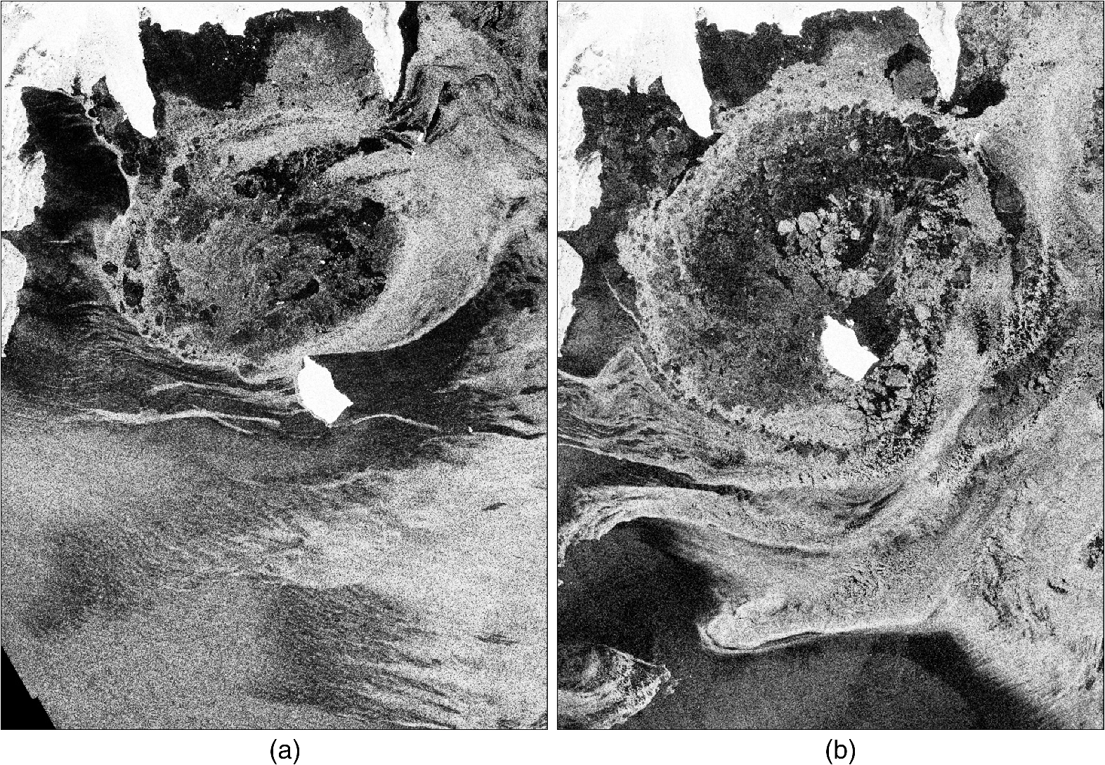
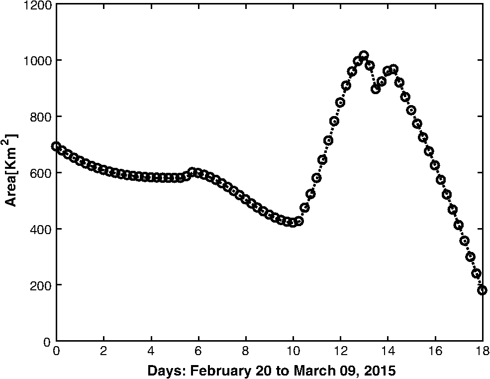
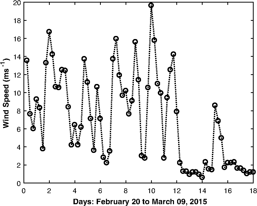
1.IntroductionThe area of Terra Nova Bay (TNB), Antarctica, has been of particular interest for the Italian scientific community in the last 30 years as the Italian Antarctic base Mario Zucchelli Station (MZS) is located in its vicinity. Thanks to the synthetic aperture radar (SAR) imagery of the area available today, a study of the dynamics of ice formation at TNB was planned for summer 2015. The European Space Agency (ESA) Third Party Mission program, which provides Cosmo-SkyMed (CSK) and Radarsat-2 (R-2) images, was used to carry out the study. A total of 14 CSK and 14 R-2 images for the period of February 20 to March 20 were retrieved; in addition, Sentinel-1 (S-1) images were also downloaded from the ESA scientific data hub. Wind data from the automatic weather station (AWS) “Eneide,” located in the vicinity of MZS, were obtained from the Italian Antarctic Research Program1 as an ancillary data set. The first survey of the SAR images revealed an unexpected surface feature, i.e., the presence of a prominent ice eddy. Ocean eddies have been found to play a major role in heat and salt transport2 and in water mass transport.3 For example, discrete eddies may account for up to 60% of the eddy kinetic energy in strong eddying currents, such as the Antarctic circumpolar current (ACC).4 Field studies have also shown that discrete eddies have a major impact on biological productivity.5 A recent study6 provided an eddy census data set from a global ocean simulation over a period of 7 years and showed that the ACC is the region with the largest number of eddies in the world. Satellite remote sensing provides a variety of platforms and sensors for monitoring sea surface and sea–atmosphere interactions and is therefore useful for observing mesoscale eddies, which may reach horizontal scales above 100 km and time periods from days to weeks. A marked variation of the sea surface temperature (SST) is one of the clearest indications of an eddy. Exploiting this feature, a neurofuzzy eddy detector was implemented with morphological descriptors, using the SST patterns of optical/infrared Nation Oceanic and Atmospheric Administration Advanced Very High Resolution Radiometer (NOAA AVHRR) images.7 In another study, the eddy shape was detected from the specific geometric structures of the rotating SST thermal wind velocity field.8 Vertical displacements of the sea surface are sensed by radar altimeters. Using the pattern of sea surface level anomaly (SLA), the eddy core area was detected with a set of specific delineation rules;9 in this case, the accuracy of the detection is limited by the heuristic function of the geometric criteria. Another proposed method combines the SLA gradient with a map of spatial markers for solving the Watershed transform.10 Although it can observe only large-scale singularities, the radar altimeter is widely used in oceanography. Combining SST and altimeter data with the geophysical knowledge of a particular site leads to a marked improvement in eddy detection. In SAR imaging, the surface variations produced by the eddy’s revolving motion yield a modulation of the backscattered signal. Similarly, with a favorable wind speed, the surface films can enhance the imaged contrast of the eddy filaments. Tracking the signature of sea surface films can be performed by maximum cross correlation or by optical flow techniques;11 in addition, the detection of slick patterns can be complemented by visual criteria.12 In changing environmental conditions, the capacity of SAR to reveal eddy singularities by sensing the usual manifestations (sea surface roughness or marine surface films) is a challenging task. For this reason, synergic SAR modeling may include complementary data, such as SST imagery, radar altimetry, ground truth measurements, and chlorophyll observations.13 European satellites provide SAR images operating in C- and X-band: as these images are free, they were chosen for this study. Recent papers have shown that C- and X-band images in HH polarization are the most effective in sea-ice detection.14,15 C- and X-band often display very similar distributions; but, when comparing their performances in discriminating the different kinds of sea ice, Dierking16 found that, only in the case of very thin ice, X-band is superior to C-band. Where the L-band is concerned, it was demonstrated its greater ability in detecting ridges and other sharp ice structures, but its lower sensibility to microscale ice structures.17 Sea-ice conditions usually have a dynamic evolution, a circumstance that may introduce ambiguities between different SAR frequency bands; in any case, Robinson18 estimates that no more than a few percent ( to 5%) of all ocean SAR images, captured in different bands, reveal substantial mesoscale features. The first part of the paper deals with the detection of a time-varying ocean eddy in SAR images, exploiting a specific example of the singularity: rather than using the radar signal, the analysis is carried out by an indirect solution, which extracts the vortex extent outlined by the floating ice fragments of the scene. This is an alternative method compared with those used in previous surveys. The task to be carried out is the identification of the eddy structure and the extraction of its main parameters: area and lifetime. In our case, from the sequence of SAR images in which the eddy was last seen on 9th March, its lifetime was about 20 days; indeed, from the image of March 15th, the ice eddy appears to be completely disrupted, and a well-defined polynya comes into sight. With regard to eddy area, a specific image processing scheme was developed. The scheme consists of the following stages: (1) nonlinear filtering, (2) segmentation, based on the Markov random field (MRF) theory, using a contextual approach applied both to the original and to the filtered image, and (3) extraction of the eddy area using an active contour detection algorithm, which works in an iterative manner. The second part of the paper focuses on the role of the katabatic wind of TNB in generating the eddy singularities. It is well known that small-scale eddies, such as those produced at high latitudes, can be generated by atmospheric forcing;19 in this paper, the correlation between Eneide wind data and eddy extent is quantified as a joint function by means of two different statistical functions. The analysis provides elements for evaluating the temporal matching of the two variables. 2.MethodsFirst, the SAR images were preprocessed using TeraScan software:20 all the images were projected onto a common geographical reference with a pixel size of 100 m. Figure 1 shows one example of a georeferenced image. From each georeferenced image, a subset, or imagette, covering the area of TNB, was extracted; a pair of these imagettes are shown in Fig. 2. Fig. 1Georeferenced Sentinel-1 image of February 25, 2015, TNB, after being remapped onto an equidistant cylindrical projection. 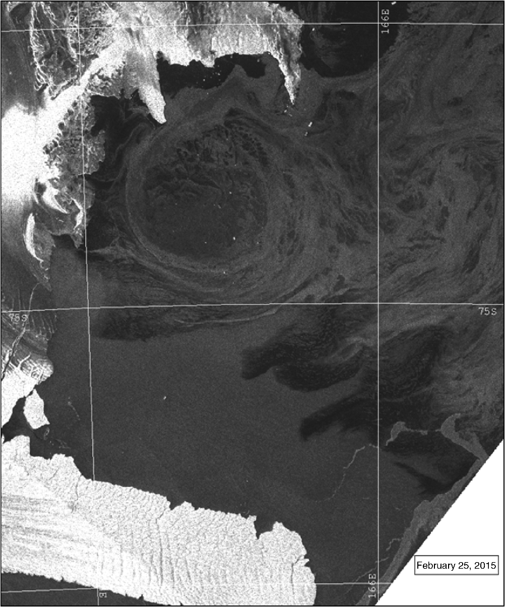 2.1.Filtering by Morphological ReconstructionAs SAR images are degraded by speckle noise, the identification of the elements of an SAR scene is a complex task. Both classical21 and adaptive filters22,23 are able to remove only a limited amount of speckle degradation in the proximity of the contour regions. The result is a blurred detection. In the first stage, concepts of gray-level morphology were applied to preserve contour information. The aim is to obtain a scene image, which is less degraded by speckle and integrated into more homogenous regions. Based on a well-defined algebra, mathematical morphology24 is a powerful tool for describing topological structures. Basic structuring shapes are the elements for defining the logical operations of morphological set theory. Two important operations are erosion and dilation, which are defined using the original image and a structuring element . The coordinates and the gray level define a space. The erosion of the image by the structuring element is the operation: , where and . Similarly, the dilation of the image by the structuring element is the operation: , where and . In both operations and are the domains of and , respectively. Erosion and dilation can be applied in a given sequence to enhance or eliminate image structures. Its combined use defines the opening (an erosion followed by a dilation) and closing (a dilation followed by an erosion) operations. Both procedures have specific interpretations. For example, the opening operation smooths contours and interrupts narrow sets of pixels, and an opening followed by a closing defines an elementary smoothing process. Mathematical morphology provides the basic theory to design nonlinear filters, which are suitable, for example, for detecting edges or revealing specific patterns. One case of interest is when the grayscale “morphological reconstruction”25,26 takes into account a “marker” image , a mask image , and a structuring element , defining a four- or eight-pixel connectivity matrix. The morphological reconstruction consists of the iterative dilation operation where and , and at the last dilation, the reconstruction is .In a practical implementation, the reconstruction can be performed taking advantage of the morphological characteristics of the opening operation. The resulting “opening by reconstruction of erosion” or just “opening by reconstruction” of the SAR image is defined as . Thus, the variables of Eq. (1) are the image and the result of the erosion operation, which is the reference marker . At this stage, the visual effect is that the crucial structures eroded by the initial operation can be fully recovered. As the opening and the closing operations affect the bright and the dark elements, respectively, the sequential use of this filter can define a more suitable smoothing filter called opening–closing reconstruction , where Eq. (1) is also applied for reconstruction. The structured elements of image are affected by the size and shape of the array. Depending on the structure of the scene features, the element applied in this paper is a flat disk-shaped structuring element defined by a five-pixel radius. As a result, small, bright, and dark features are reduced, and the contours of the primary regions are reconstructed well. This is a simple but functional process for soft filtering the random behavior of the speckle. 2.2.SegmentationIn the second stage, the scene is modeled by means of MRF theory. To define the conditional probability in terms of the Bayesian equation, the proposed algorithm analyzes the information derived from the gray-level data. With this scheme, the a priori model implements a homogeneity criterion based on the local label distribution. The segmentation result is obtained by a recursive stochastic minimization scheme. Before seeking the eddy boundary, the scene data require topological conformation, which means we need to have a clean space inside the eddy area, that is, we need to detect and remove the sea-ice objects located inside. This assignment is carried out by a hierarchical labeling process, defined by the topological properties of the ice fragments. Next, the eddy contour extraction task is performed. The geometry of the eddy is not regular and is usually defined by nonclosed contour segments. Classical edge detection algorithms are not very useful because of the complex contour distribution. To overcome this problem, an active contour detection algorithm is used. Moving in an iterative way, the active contour is placed according to both the gradient and the segmented image information. The final result is a binary mask, which provides the detection of the closed form of the eddy. In this way the final size of the eddy area is derived. Let us consider two random variables, and . In a maximum a posteriori (MAP) approach, let be the image to be segmented and be the segmentation result, , where is the number of labels of the sample space. The Bayesian rule is applied to define the equation of the segmentation model , where the joint probability term is . As the total probability of is a common term throughout the process, a simpler expression is obtained by making this term equal to 1. The resulting expression is . The segmentation problem can be considered as a probabilistic labeling process. According to the Bayes theory, the MAP estimation equation can be written as , where is the label field to be estimated. The Markov hypothesis makes the assumption that both fields and are expressions of MRFs, and, in this case, the Gibbs probability distribution27 can be used to represent the terms of the Bayes estimation. The Gibbs distribution follows an exponential law; hence, the resulting Markovian estimation equation is where the probability that a given pixel belongs to a particular label is derived by minimizing the a posteriori energy function . In this paper, the conditional energy term is estimated using the pixel gray-level information, and the a priori law is achieved by a contextual analysis of the local label structure.To define the information provided to the conditional energy term, the proposed algorithm considers both the original image and the filtered one . The morphological filtering performs an important noise smoothing task; but, depending on the topology of the structuring element , thickening or removal of small objects may occur in connected regions, with a shifting of the image features. Some important information still remains in the raw image, and it can be used to complement the segmentation process. An interesting alternative to the combined use of information sources arises when one considers the probability property of independence28 as being conditioned by the field of labels. The probability of the joint gray-level information of pixels and , given the label , is obtained by the product rule: . Including the former property in the Markovian model, Eq. (2) is approximated as where is the conditional energy function of the gray-level occurring given the label. This equation involves the conditional random field of the two-level model. In addition, and are the weight coefficients of the conditional membership functions. With these coefficients, it is now possible to assess the energy contributions of images and .To define the a priori energy function , the Ising model is used; the Hamiltonian is then given by , where is the strength of interaction of the ferromagnetic model and when pixels at coordinates and of the segmented image have the same label . To define homogeneous regions, the minus sign supports the minimization process in Eq. (3). Binary segmentation is required to detect the scene elements. The MRF model provides the required binary field by labeling the set of pixels as ice or nonice (open sea). The segmentation result is obtained by a simulated annealing scheme.29 Using , the convergence is achieved by applying a number of 35 iterations, with a strength parameter . As an example of the preprocessing steps, Fig. 3 shows the results obtained with the nonlinear filter (a) and using the binary Markovian segmentation (b). These results were obtained with the CSK image of March 5th [Fig. 2(b)]. 2.3.Toward Eddy Region BoundingThe MRF segmentation provides a binary result, where the background of the SAR scene is displayed as black pixels for the open-sea regions and as white pixels of the detected sea-ice objects. Some dynamic characteristics of the wind can be seen in the spatial distribution of the sea-ice elements; this wind signature is easily detected as these elements form a sort of ring. The sea-ice objects do not define a perfect circle (see Figs. 2 and 3) as its contours are nonstationary. To complete the scene description, we must deal with a number of minor sea-ice fragments, which can be seen inside the eddy area; they are not part of the eddy topology and can lead to spurious detections. Before completing the detection and the extraction of the eddy contour, it is important to remove these sea-ice fragments from the scene; to achieve this goal, the ice objects are classified using a labeling method. Graph theory30 provides useful concepts for describing the objects of a scene. A graph is defined as the set , where is a set of “vertices,” and is a set of “edges.” In our case, the set of vertices refers to the lattice structure of the image, and the set of edges is formed by linking pairs of pixels of the set . One way of characterizing the edge features is done by describing the “adjacency” and “connectivity” of set . Two pixels are four-adjacent when they share a side. A set of pixels is defined as connected when it is not divided by a boundary. A region is called four-connected or if a finite chain links every pixel to a set of consecutive four-neighbor pixels. The provides an important relationship for labeling segmented scenes. An “ordering list” is arranged for labeling the four-connected regions,31 and the number of pixels of each object is obtained. A percentage of the image size is used to fix a threshold . When , the related sea-ice object is removed. Figure 4 shows the result of applying this process to the CSK imagette of March 5th. A spotless area is observed inside the eddy [Fig. 4(b)], and the scene is now suitable for deriving the eddy boundary. 2.4.Extraction of Eddy AreaThe next stage performs the detection of the eddy boundary and the extraction of its area. On binary images, background and foreground objects are very well defined; consequently, pixel-based edge detection algorithms produce excellent results.32,33 A serious challenge is to extract and link the contour segments that define the closed form of the eddy contour from the contour set of the whole image. Medicine and biology imaging often deal with curvilinear objects. Some well-known techniques, which are useful for object representation, feature extraction, and parametric contour description of circular and elliptical objects. A direct least-squares fitting method34,35 was proposed to trace the boundary of an elliptical object. By minimizing the ellipse constraint, these methods claim to be invariant to affine transformations. The Hough transform is another way of detecting regular shapes. In another case,36 the minimum and maximum radii were manually drawn in an edge map of an embryo image. Some circular forms lie in the image, and each pixel of the edge map is considered as a potential element of a circle. A systematic scan by the Hough transform detects the circular structures with a size defined by the radius range. The result is a set of potential circles but with spurious findings. Thus, further supervised validation is required. The main drawback of this boundary analysis is that the geometry of the eddy is not regular as it is formed by the connected contour segments of several sea-ice objects; this means that fitting its boundary to a circle or an ellipse is only a rough approximation. Thanks to the parametric representation, a formal basis for the boundary analysis of the eddy extent can be provided. To solve our problem, an active contour detection algorithm37 is applied. Moving in an iterative way,38 a pixel-based template develops, based on both the gradient and the segmented image information, evolving toward the boundary of the eddy. A parametric closed curve defines the deformable model by a set of coordinates , where is the normalized length boundary of the active contour. The deformation process is modeled using terms as follows: (i) internal energy , which makes the template regular; (ii) external energy, which leads the template toward the regions of high gradient ; and (iii) external constraint forces for manual regulation by the user. The total energy function is given by The internal energy is described by , where , , , and are the terms of elasticity, rigidity, and the first- and second-order spatial derivatives of the curve , respectively. is the closed contour of the snake. The elastic energy is modeled by , and the bending energy is controlled by . To compute the derivatives, the energy function is discretized by a finite difference method. The image energy, , leads the snake to the edge regions using a gradient operator. The constraint energy, , allows manual intervention by the user, assigning attractive or repulsive operators to specific regions. An initial pixel-based template is manually placed near the eddy boundary. Equation (4) is minimized, and the curve evolves until it fits the eddy shape. The spline iteratively moves into pixels with lower energy, seeking a better match to the nearest edges. The spline pixels are updated by , where is the solution at a given iteration, which is perturbed by a small deviation . The information required by the energy term can be provided by the rate of change of the gray level, which is usually computed by the gradient operator by means of the partial derivatives. Instead of implementing the gradient operator with spatial convolution, we propose to express the image energy term using the discrete formulation of the morphological gradient . is thus given by the morphological operators: dilation and erosion , where is the binary segmented image. The active contour algorithm was applied to the set of imagettes with the eddy area free of sea-ice fragments, as obtained in Sec. 2.3. To enhance the detection procedure, the imagette of March 5th is used as a reference: in Fig. 4(a), the closed form of the eddy is shown in blue color using the remapped SAR image, and in Fig. 4(b) with the binary eddy area free of sea-ice objects. 3.ResultsThe eddy area values are shown in Fig. 5. They were obtained using the processing scheme described above as applied to the sequence of imagettes extracted from CSK, R-2, and S-1 images. The interaction between variables can be computed by measuring the degree of relationship with the assumption of linear or nonlinear dependence. To reveal the coupling between the forcing wind and the induced eddy area, with an alternative perspective, we preferred to analyze the case of a linear relationship by means of two formal statistical correlation functions. The examination is derived from the time series analysis used to provide explicit indicators of the dependence on wind field. To quantify the linear interaction between geophysical processes and meteorological variables, the running correlation coefficient function39 is simply the adoption of the second-order statistic moment of a bivariate random variable. Using local windows overlapped in time, the function is the first analysis method. Let be the total data length; , the wind speed; and , the measured eddy area; the of the two centered signals, given the ’th step with a window length , is computed using both first- and second-order moments of the marginal variables where is the expected value computed with the window width . The total length of the evaluation is , which shows the time evolution of the linear interaction between the discrete series variables.In the second analysis, we propose to apply the Spearman correlation coefficient,40 which is a nonparametric rank statistic measure of the connection between variables. One important feature of this function is that it is less affected by single influential observations (outliers). The central information provided by this function is the monotone dependence between variables. Using the same moving window of the function, a high correlation value means that both variables have corresponding increasing or decreasing distributions. This may seem a simple feature; but, it is another element that demonstrates the association involving the two time series. The “monotonic relationship” of the Spearman correlation complements the “linear dependence” displayed by the function. The AWS Eneide, located on TNB near MZS, collects the wind channeled by the mountains of the inner continent (see Fig. 1) and provides real-time and archived meteorological data. Wind speed and direction of Eneide were composed in one single figure defined as “effective wind field,” i.e., the wind component pushing eastward or at 270 deg. The acquired data are transmitted by the Argos satellite every hour and received in Italy. For the 18-day study period, February 20 to March 9, the collected wind field is shown in Fig. 6 (each value is the average over the previous 6 hrs). The final step is the statistical inference of the dependence between the two variables. The pairwise linear correlation function was analyzed by Eq. (5) using bounded temporary windows. This function makes it possible to explain the interaction of the geophysical variables in discrete time series. Using a time lag of , is computed with windows of 5 units (time segment of 30 hr); the result is shown in Fig. 7(a). The result of the Spearman correlation is shown in Fig. 7(b). Both variables, eddy extent and wind speed, can be considered as random variables, but a joint connection is observed. Figure 7 shows that 57% of the coefficients have a correlation , which, using statistical criteria, confirms both a strong linear relationship and a monotone association between the two variables. Fig. 7Correlation functions between eddy extent and wind speed: (a) the running correlation coefficient and (b) the Spearman correlation coefficient. 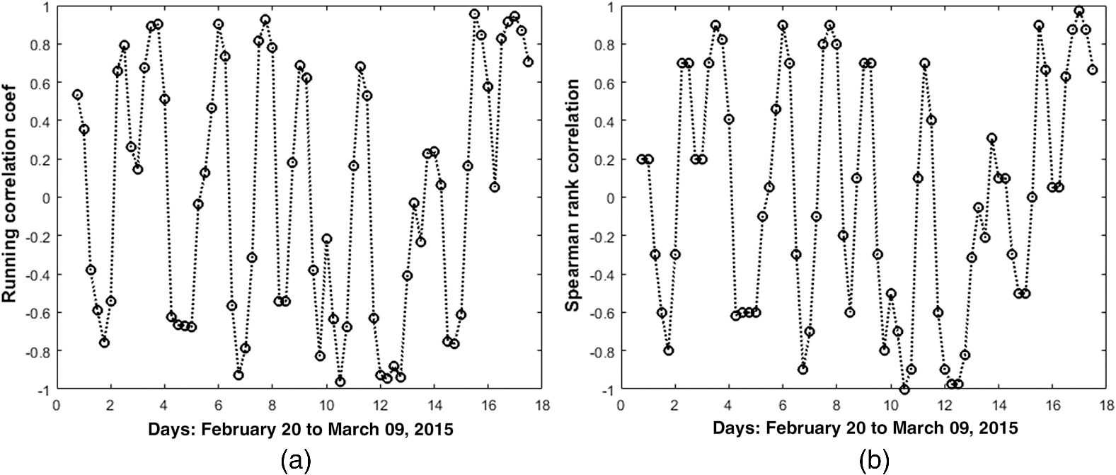 By statistical criteria, a very strong correlation arises when . Figure 7 shows that only 26% of the paired data are very strongly correlated. The probability theory states that two random variables are independent when the occurrence of one variable does not affect the manifestation and the evolution of the second one, and, consequently, the variables are uncorrelated. Given that strong and very strong correlations are widely distributed, our results show that the analyzed variables are not statistically independent. It is well known that eddies can be induced by other geophysical events, such as the interaction of sea currents with undersea topography, or by convection caused by the sea surface gradient temperature. Related information of such events was not available for this study; nevertheless, the correlation sequence reveals a dependency between wind field and eddy extent variation. 4.DiscussionIdentifying eddy singularities in SAR images is only a partially solved problem given the complex signature of the sea/atmosphere modulation pattern. For this reason, the analysis of the scene features requires a specific processing procedure as suggested by the present paper. Based essentially on the Bayesian estimation and on the MRF theory, an original aspect of the proposed scheme consists of a methodology to parametrize the eddy structure, to detect its temporal evolution in the time window of 18 days. The advantage of our proposal is that the contextual dependence of the segmentation process model is able to deal with the noisy behavior of the images from different satellites (CSK, R-2, and S-1). The resulting scene characterization is provided by merely binary labeled fields, see Fig. 3(b); this seems a simple outcome, but a functional product cannot be obtained by conventional segmentation methods. Two objective correlation measures are used to prove the correspondence between the geophysical variables involved. Both ocean and atmospheric dynamics impact the floating ice distribution, and this introduces discrepancies in the traced eddy contour. The detection of ice fragments floating in the surrounding environment, being configured by a set of segments, is not very precise and yields some divergence in the correlation progression, see Fig. 4. A clear limitation of the correlation measure is that the statistical interpretation is only a “linear” one, whereas a nonlinear analysis is beyond the scope of this paper. The recursive structure of the MRF algorithm requires a significant amount of processing time: using MATLAB® and computing with an Intel Pentium® CPU G2020 of 2.9 GHz and 6 GB RAM memory, the elapsed time for a single scene is about 1150.1 s. 5.ConclusionsEddies play an important role in the dynamic distribution of heat, mass, and other geophysical variables, which operate at high latitudes. This paper presents a complex processing scheme developed to model small-scale eddies generated by atmospheric forcing. First, a nonlinear filter is applied to a sequence of imagettes extracted from the SAR images; the filter task is the smoothing of the speckle degradation while preserving primary details. The filtering stage is complemented by a segmentation stage based on MRF theory. Because of the speckle effect, the use of both filtering and MRF stages provides a contextual analysis, which improves the segmentation result. Two regions of the imagettes are considered for the purposes of this paper: the open sea and the sea-ice, both regions being delimited as objects, and with the floating ice providing basic information for tracing the eddy bounds. The set of sea-ice objects of the binary segmentation is labeled to remove drifting sea-ice objects from the internal eddy region. Using this criterion, small objects, both inside and outside the eddy, are rejected, even though the primary interest is to remove those inside the eddy. In this way, a clear definition of the eddy boundary is obtained. The use of an active contour algorithm enhances the overall quality of eddy extent detection. The processing scheme presented in this work, when applied to the set of SAR images of TNB, produces a database of area variation in the study period. The link between eddy area and wind field was analyzed by means of the running correlation coefficient function () and the Spearman correlation coefficient, which revealed the soundness of the linear relationship and the monotone dependence between the two variables. AcknowledgmentsThe authors wish to thank the ESA for providing SAR images through the Third Party Mission Program: CSK to F.P. (Project Proposal id14674) and Radarsat-2 to C.F. (Project Proposal id1652). We also thank the Meteo-Climatological Observatory of the Italian Program for Antarctic Research1 for providing wind data collected by the AWS Eneide. We acknowledge the support of the EU SPICES project41 to F.P. and L.G., and of the Direccion General de Asuntos del Personal Academico, Program PASPA–UNAM, to M.M.F. Finally, the authors wish to thank the anonymous reviewers who provided useful comments on a previous version of this paper. ReferencesAntarctic Meteo-Climatological Observatory, “Profiles of wind, MZS,”
(2017) www.climantartide.it June ). 2017). Google Scholar
A. Chaigneau et al.,
“Vertical structure of mesoscale eddies in the eastern South Pacific Ocean: a composite analysis from altimetry and Argo profiling floats,”
J. Geophys. Res., 116
(C11), 1
–16
(2011). http://dx.doi.org/10.1029/2011JC007134 Google Scholar
A. M. Doglioli et al.,
“Tracking coherent structures in a regional ocean model with wavelet analysis: application to Cape Basin eddies,”
J. Geophys. Res., 112
(C5), 1
–12
(2007). http://dx.doi.org/10.1029/2006JC003952 Google Scholar
D. B. Chelton et al.,
“Global observations of large oceanic eddies,”
Geophys. Res. Lett., 34
(15), 1
–5
(2007). http://dx.doi.org/10.1029/2007GL030812 GPRLAJ 0094-8276 Google Scholar
J. D. Everett, M. E. Baird and I. M. Suthers,
“Three-dimensional structure of a swarm of the salp Thalia democratica within a cold-core eddy off southeast Australia,”
J. Geophys. Res., 116
(C12),
(2011). http://dx.doi.org/10.1029/2011JC007310 Google Scholar
M. R. Petersen et al.,
“A three-dimensional eddy census of a high-resolution global ocean simulation,”
J. Geophys. Res., 118
(4), 1759
–1774
(2013). http://dx.doi.org/10.1002/jgrc.20155 Google Scholar
J. A. Piedra-Fernandez et al.,
“Fuzzy content-based image retrieval for oceanic remote sensing,”
IEEE Trans. Geosci. Remote Sens., 52 5422
–5431
(2014). http://dx.doi.org/10.1109/TGRS.2013.2288732 IGRSD2 0196-2892 Google Scholar
C. Dong et al.,
“An automated approach to detect oceanic eddies from satellite remotely sensed sea surface temperature data,”
IEEE Trans. Geosci. Remote Sens. Lett., 8 1055
–1059
(2011). http://dx.doi.org/10.1109/LGRS.2011.2155029 Google Scholar
J. Yi et al.,
“Automatic identification of oceanic multieddy structures from satellite altimeter datasets,”
IEEE J. Sel. Top. Appl. Earth Obs. Remote Sens., 8 1555
–1563
(2015). http://dx.doi.org/10.1109/JSTARS.2015.2417876 Google Scholar
L. Qin et al.,
“A new method for mesoscale eddy detection based on watershed segmentation algorithm,”
Proc. SPIE, 9261 92610A
(2014). http://dx.doi.org/10.1117/12.2069167 Google Scholar
L. Dreschler-Fischer et al.,
“Detecting and tracking small scale eddies in the black sea and the baltic sea using high-resolution Radarsat-2 and TerraSAR-X imagery (DTeddie),”
in IEEE Geoscience and Remote Sensing Symp.,
1214
–1217
(2014). http://dx.doi.org/10.1109/IGARSS.2014.6946650 Google Scholar
S. Yamaguchi and H. Kawamura,
“SAR-imaged spiral eddies in Mutsu bay and their dynamic and kinematic models,”
J. Oceanogr., 65
(4), 525
–539
(2009). http://dx.doi.org/10.1007/s10872-009-0045-5 JOOCE7 0916-8370 Google Scholar
A. Y. Ivanov and A. I. Ginzburg,
“Oceanic eddies in synthetic aperture radar images,”
J. Earth Syst. Sci., 111
(3), 281
–295
(2002). http://dx.doi.org/10.1007/BF02701974 Google Scholar
M. Moctezuma, F. Parmiggiani and L. Lopez,
“Automatic measurement of Polynya area by anisotropic filtering and Markova random fields,”
IEEE J. Sel. Top. Appl. Remote Sens., 7
(5), 1665
–1674
(2014). http://dx.doi.org/10.1109/JSTARS.2014.2314684 Google Scholar
M. Moctezuma-Flores and F. Parmiggiani,
“Tracking of the iceberg created by the Nansen Ice Shelf collapse,”
Int. J. Remote Sensing, 38
(5), 1224
–1234
(2017). http://dx.doi.org/10.1080/01431161.2016.1275054 IJSEDK 0143-1161 Google Scholar
W. Dierking,
“Sea ice classification on different spatial scales for operational and scientific use,”
in Proc. of ESA Living Planet Symp.,
(2013). Google Scholar
L. E. Eriksson et al.,
“Evaluation of new spaceborne SAR sensors for sea-ice monitoring in the Baltic Sea,”
Can. J. Remote Sens., 36
(Suppl. 1), S56
–S73
(2014). http://dx.doi.org/10.5589/m10-020 CJRSDP 0703-8992 Google Scholar
I. S. Robinson,
“Mesoscale ocean features: eddies,”
Discovering the Ocean from Space: The Unique Applications of Satellite Oceanography, 69
–114 Springer, Berlin, Heidelberg
(2010). Google Scholar
W. Alpers, D. Dagorne and P. Brandt, Satellite Observations of Oceanic Eddies Around Africa, 205
–229 Springer Netherlands, Dordrecht
(2014). Google Scholar
SeaSpace Corporation, “TeraScan® satellite processing systems21,”
(2017) www.seaspace.com June ). 2017). Google Scholar
J. S. Lee,
“Speckle suppression and analysis for synthetic aperture radar,”
Opt. Eng., 25
(5), 255636
(1986). http://dx.doi.org/10.1117/12.7973877 Google Scholar
A. Baraldi and F. Parmiggiani,
“A refined gamma MAP SAR speckle filter with improved geometrical adaptivity,”
IEEE Trans. Geosci. Remote Sens., 33
(5), 1245
–1257
(1995). http://dx.doi.org/10.1109/36.469489 IGRSD2 0196-2892 Google Scholar
A. Yommy, R. Liu and S. Wu,
“SAR image despeckling using refined Lee filter,”
in 7th Int. Conf. on Intelligent Human-Machine Systems and Cybernetics (IHMSC),
260
–265
(2015). Google Scholar
J. Serra and L. Vincent,
“An overview of morphological filtering,”
Circuits Syst. Signal Process., 11
(1), 47
–108
(1992). http://dx.doi.org/10.1007/BF01189221 Google Scholar
O. Marques, Practical Image and Video Processing using MATLAB, Wiley-IEEE Press, Hoboken
(2011). Google Scholar
R. C. Gonzalez and R. E. Woods, Digital Image Processing, 3rd ed.Prentice-Hall Inc., Upper Saddle River
(2008). Google Scholar
O. Ibe, Markov Processes for Stochastic Modeling, 2nd ed.Elsevier Science, London
(2013). Google Scholar
A. Papoulis and S. U. Pillai, Probability, Random Variables and Stochastic Processes, 4th ed.McGraw-Hill, New York
(2002). Google Scholar
S. Z. Li, Markov Random Field Modeling in Image Analysis, 3rd ed.Springer-Verlag, London
(2009). Google Scholar
S. Theodoridis and K. Koutroumbas, Pattern Recognition, 4th ed.Academic Press, Burlington
(2009). Google Scholar
E. Gose, R. Johnsonbaugh and S. Jost, Pattern Recognition and Image Analysis, Prentice-Hall Inc., Upper Saddle River
(1996). Google Scholar
S. T. Bow, Pattern Recognition and Image Preprocessing, 2nd ed.CRC Press, New York
(2002). Google Scholar
W. Pratt, Digital Image Processing: PIKS Inside, 3rd ed.John Wiley & Sons Inc., New York
(2001). Google Scholar
A. Fitzgibbon, M. Pilu and R. B. Fisher,
“Direct least square fitting of ellipses,”
IEEE Trans. Pattern Anal. Mach. Intell., 21
(5), 476
–480
(1999). http://dx.doi.org/10.1109/34.765658 ITPIDJ 0162-8828 Google Scholar
X. Ying et al.,
“Direct least square fitting of ellipsoids,”
in 21st Int. Conf. on Pattern Recognition (ICPR),
3228
–3231
(2012). Google Scholar
O. Demirkaya, M. H. Asyali and P. K. Sahoo, Image Processing with MATLAB: Applications in Medicine and Biology, CRC Press, Boca Raton
(2008). Google Scholar
M. Kass, A. Witkin and D. Terzopoulos,
“Snakes: active contour models,”
Int. J. Computer Vision, 1
(4), 321
–331
(1988). http://dx.doi.org/10.1007/BF00133570 IJCVEQ 0920-5691 Google Scholar
J. Montagnat, H. Delingette and N. Ayache,
“A review of deformable surfaces: topology, geometry and deformation,”
Image Vis. Comput., 19
(14), 1023
–1040
(2001). http://dx.doi.org/10.1016/S0262-8856(01)00064-6 Google Scholar
K. Kodera,
“Quasi-decadal modulation of the influence of the equatorial quasi-biennial oscillation on the north polar stratospheric temperatures,”
J. Geophys. Res., 98
(D4), 7245
–7250
(1993). http://dx.doi.org/10.1029/92JD02930 Google Scholar
M. R. Spiegel and L. J. Stephens, Schaum’s Outline of Theory and Problems of Statistics, McGraw-Hill, New York
(2007). Google Scholar
Space-borne observations for detecting and forecasting sea ice cover extremes, SPICES, “Horizon 2020 European Union Program,”
(2017) www.h2020-spices.eu/ June ). 2017). Google Scholar
BiographyMiguel Moctezuma-Flores received his BS and MS degrees in electrical engineering from the National University of Mexico (UNAM) in 1985 and 1988, respectively, and his MSc and PhD degrees in image processing from the National Higher School of Telecommunications, Paris, France, in 1991 and 1995, respectively. He was a visiting fellow with the Italian National Research Council (CNR), Bologna, Italy, in 2016. He is a professor in the Telecommunications Department of the Engineering School, UNAM. Flavio Parmiggiani received his Laurea degree in physics from the University of Milan, Italy, in 1970. He has been a researcher at CNR from 1973 to 1989, a prime researcher from 1989 to 2001, and a director of research at ISAC from 2001 to date. From 1989 to 2014, he was responsible for the satellite receiving station at the Italian Antarctic base Mario Zucchelli Station at TNB, Antarctica. Since 1992, he has been working on marine applications of SAR images. Corrado Fragiacomo completed his studies of electronics in 1973. He has been working at the National Institute of Oceanography since 1982, and his work has been related to remote sensing using the satellite receiving station for polar orbiting satellites since 2000. He took part in eight Antarctic Campaigns, responsible for the Remote Sensing Laboratory of the Italian base. He is currently involved in research projects using satellite SAR data. Lorenzo Guerrieri received his MS degree in physics from the University of Modena and Reggio Emilia, Modena, Italy, in 1999 and his PhD in geophysics from the University of Genova, Genova, Italy, in 2006. He collaborated with the Italian National Institute of Geophysics and Volcanology, Rome, Italy, working on volcanic atmospheric emission from satellite spectral radiance measurements. He is currently working with CNR-ISAC, Bologna, Italy, on polar sea ice from SAR images. |