|
|
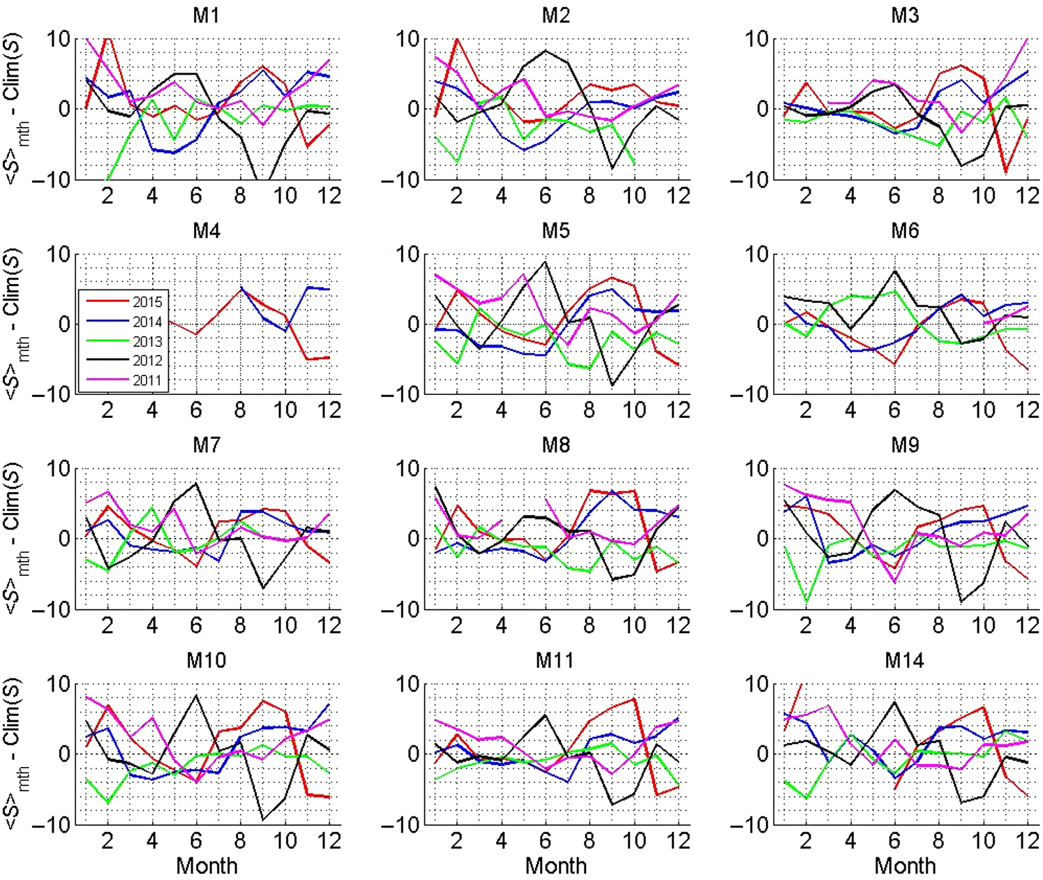
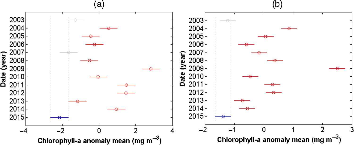
1.IntroductionThe CONsortium for oil spill exposure pathways in COastal River Dominated Ecosystems (CONCORDE) studies the ecosystem dynamics and characterization of the complex four-dimensional physical, geochemical, and bio-optical fields in the Mississippi Bight influenced by pulsed river discharge. A key question addressed by CONCORDE is: Despite the fluvial input into the Mississippi Sound (MSS) and Mobile Bay [Fig. 1(a)], how can oil and other pollutants enter the Sound and Bay from the shelf and reach the coastal mainland, as it did during the Deepwater Horizon (DWH)/Macondo Well oil spill?1 This study focuses on a particular set of meteorological events that resulted in shelf waters being forced into the MSS, and so provides a scenario where an offshore oil spill or other toxic events, could affect the MSS and coastal mainland. Fig. 1(a) Study area map with MDMR/USGS stations (black labels) and NOAA/NDBC stations and buoys (red labels) in the Mississippi Bight. Contour lines represent the isobaths. The red dotted lines represent the transects used to extract the chlorophyll-a anomalies from MODIS-Aqua. Blue lines on land represent the rivers. (b) The track of Patricia’s remnants over the southern United States. Black box denotes the study area. 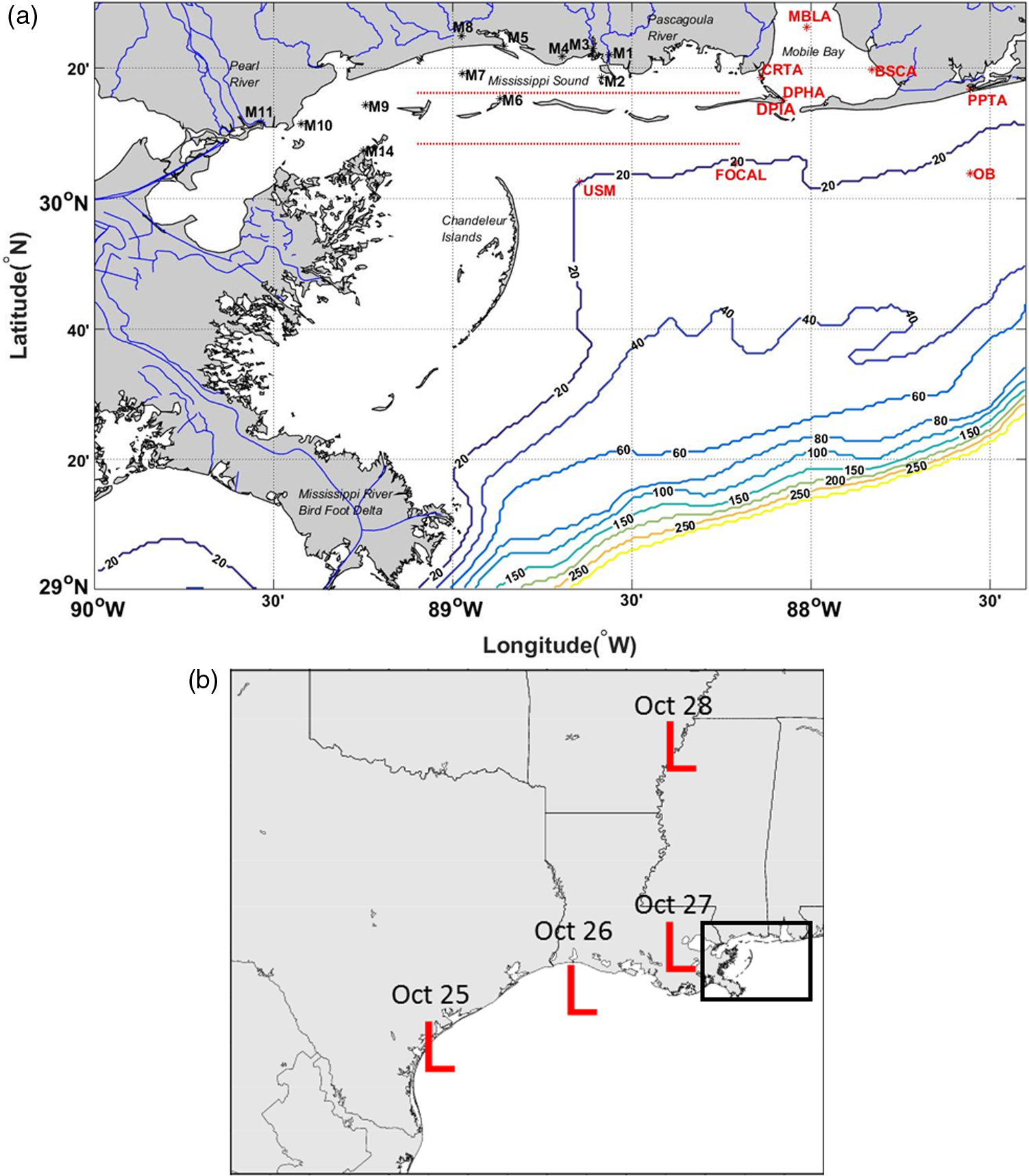 The first CONCORDE cruise occurred on October 27 to November 7, 2015, shortly after the passage of tropical cyclone Patricia’s remnants over the study area. Patricia had dissipated over the Sierra Madre mountains in Mexico after its landfall on the coast of southwestern Mexico as a category four hurricane, but interacted with an upper-level baroclinic trough, and reformed as a baroclinic cyclone.2 The cyclone moved north-northeast from south Texas to southeast Louisiana from 12:00 UTC October 25 to 00:00 UTC October 27, 2015, then turned north paralleling the Louisiana/Mississippi state line until 00:00 UTC October 28, 2015 [Fig. 1(b)]. After it reached northwest Mississippi, the system moved east over north Alabama. The unusual path created wind patterns favorable to storm surge water elevations of 0.6 to 1.2 m in coastal Louisiana, Mississippi, and Alabama. By 00:00 UTC October 30, 2015, a cold front reached the study region with widespread rainfall and shifted the winds to an offshore component, conducive to flushing estuaries such as Mobile Bay. The Navy Coastal Ocean Model (NCOM) circulation predictions and ocean color imagery from the Moderate Resolution Imaging Spectroradiometer onboard the Aqua (MODIS-Aqua) satellite were analyzed during the CONCORDE precruise preparation in October 2015 and identified strong and persistent easterly-southeasterly surface currents transporting offshore waters onto the shelf from October 18 to 26, 2015. During the same period, a prolonged inflow of saline offshore waters into the MSS and Mobile Bay occurred through the barrier island passes. This event lasted until the passage of Patricia’s remnants and subsequent frontal systems over the region and was atypical in its extended duration of more than 7 days as well as in intensity. This event occurred right before the CONCORDE cruise. Such an influx of offshore waters into coastal areas could be crucial in the case of an oil spill or a toxic phytoplankton bloom event allowing toxins to reach the crucial coastal habitats. The coastal waters of the northern Gulf of Mexico (nGoM) are characterized by rich and diverse ecosystems such as salt marshes and wetlands which are extremely valuable for nursery habitats, oyster reefs, and fisheries in general.3–5 Toxic events such as oil spill and harmful algal bloom (HAB) events are detrimental for coastal ecosystems and fisheries of the Louisiana (LA), Mississippi (MS), and Alabama (AL) coast. In the aftermath of the DWH oil spill event, oil and dispersants reached the coastline in the nGoM and resulted in environmental damage in the Gulf States.6–9 Advection of Karenia brevis HABs from the Florida Panhandle have episodically reached the MSS,10,11 and most recently a Karenia brevis bloom reached the MSS during the fall of 2015 causing the closure of oyster beds for several weeks and alerting the coastal managers of the potential implications of these episodic events. Although the MSS and Mobile Bay coastal habitats are separated from the open shelf by the barrier islands, they are not immune to advection of pollutants from offshore waters. Coastal and estuarine ecosystems can be impacted if offshore waters from the shelf are transported into the estuarine system via the barrier island inlets. Salinity levels within coastal areas of Mississippi and Alabama are generally high (, practical salinity units) in open water areas located south of the barrier islands and low () in near-coastal areas inside the MSS and Mobile Bay estuaries due to freshwater sources flowing into the systems.12–16 Total mean discharge from rivers into the Mobile Bay and the MSS is low in the fall season, so the resulting freshwater plumes onto the inner-shelf region of nGoM would be minimal.17 Although estuarine waters can impact the coastal water,18 the shelf is generally dominated by high-salinity offshore waters and westward currents during the fall months.19,20 The connection and interaction between the estuaries and shelf waters in the nGoM occur through the multiple barrier island inlets south of the mainland. Surface salinity records from stations near the barrier islands indicate that the inflow and intrusion of high-salinity Gulf of Mexico (GoM) waters into the MSS and Mobile Bay, i.e., north of the barrier islands, all along the water column occur episodically.12 In general, these saltwater inflow events are observed to be short-lived, i.e., on the order of hours and usually less than a day. However, the potential impact of oil spills, HABs, or similar events on coastal and estuarine ecosystems could be intensified if offshore shelf waters were persistently transported into these systems during such toxic events on the shelf. There have been previous studies focusing on the oceanography, hydrology, and ecology of the Mississippi Bight and Sound.15–17,21–23 The MSS is primarily a vertically well-mixed semienclosed estuary, also showing characteristics of a partially well-mixed estuary and locally a stratified estuary.12 August–October is a low-inflow/high-salinity period and the persistent southerly and southeasterly winds and low discharge cause strong vertical stratification in the Mobile Bay and MSS.17 Kjerfve24 showed that 1-week period meteorological events control water exchanges between the estuary and GoM. Wind forcing and freshwater discharge are important factors impacting the flow structure on the shelf and the transport of plume and nonplume surface waters on the shelf.25,26 Dietrich et al.27 studied surface trajectories of oil transport along the nGoM coastline with a coupled numerical model system of Simulating WAves Nearshore (SWAN) and ADvanced CIRCulation (ADCIRC) Model and showed that a hurricane landfall during an oil spill would move oil from the shelf into the MSS and toward the coastline. Zaron et al.28 showed using an ocean model that cyclones dramatically altered oil spill transport pushing oil into the Western MSS in Summer 2010 following DWH oil spill and showed that the estuarine intrusion and shoreline impacts from DWH were associated with edge influences of Hurricane Alex in late June 2010 followed by a baroclinic cyclone 1 week later. Arnone et al.29 used a combination of satellite products and physical models to show that a significant amount of offshore surface waters may exchange across the shelf moving onshore from the shelf break to the inner-shelf. Kim and Park30 studied the Mobile Bay system with a hydrodynamic modeling system and showed that along-shelf east wind events during weak-stratification conditions due to low discharge induces onshore Ekman transport and causes onshore transport of saline GoM waters. More recently, Webb and Marr31 showed that flushing in Mobile Bay may be inhibited due to increases in easterly wind speed and northerly flows along the shorelines. Many of these studies focused on the exchange between Mobile Bay and the shelf; however, studies of exchange between the MSS and the Bight have been limited. Thus the interaction and connection between the less saline, colder MSS and Mobile Bay waters, and more saline, warmer shelf waters are not fully understood, especially during inflow events when GoM waters intrude into the estuarine systems. In this study, the goal is to combine ocean model forecasting products and in situ coastal ocean measurements with ocean color satellite imagery to understand the mechanisms that bring offshore saltier waters into the MSS and Mobile Bay for extended periods. These mechanisms including coastal ocean circulation, river discharge, and meteorological forcing will be examined to improve the understanding of inflow and intrusion of shelf waters into the estuaries which could potentially bring offshore sources of oil and toxins into coastal systems. 2.Data and Methods2.1.Study AreaThe study area is within the Mississippi Bight located in the nGoM [Fig. 1(a)]. The Mississippi Bight coastal plain is broad and of low relief which allows large estuarine systems to intrude inland.15,16 This complex coastal ecosystem is defined by a series of barrier islands that separate the estuarine system from the Gulf of Mexico. The barrier islands are separated by inlets and protect the shallow lagoons of Mobile Bay, MSS, Chandeleur Sound, and Breton Sound.32 Our study focused on the MSS and Mobile Bay which have water depths less than 6 m and a mainly diurnal tide of less than 0.6 m. The MSS is a shallow (average 3-m deep) elongated estuarine basin that connects to the GoM through a series of passes between five barrier islands, i.e., Cat, Ship, Horn, Petit Bois, and Dauphin islands [Fig. 4].12,24,33 Although the geographical boundaries of the MSS are often a source of debate, the eastern and western boundaries are nominally Mobile Bay and Cat Island.32 Most of the fresh water fluxes into the MSS are due to the Pascagoula and Pearl rivers, however, other smaller rivers (i.e., Biloxi, Tchoutacabouffa, Jourdan, and Wolf), small bayous, and even Mobile Bay and the Mississippi River contribute to the fresh water inputs into the Sound.12,17 The Mobile River may contribute fresh water to the eastern side of the Sound, while the western MSS may receive fresh water from the Mississippi River especially when the Bonnet Carré spillway is open12,24,34 and also from other rivers through Lake Borgne and Pontchartrain. Based on salinity, Eleuterius12 defined the Sound as vertically well-mixed from July to December, with vertical homogeneity reaching a peak in October which is the period of interest. Adjacent to the MSS is Mobile Bay, a wide, shallow, and highly stratified estuary. The main freshwater sources for Mobile Bay are the Mobile and Tensaw Rivers.14 A representative monthly average salinity in Mobile Bay was recorded as 13 psu during August–October 1968 and 4 psu during February–April 1969. The monthly average representative salinity in the MSS is generally higher with an average salinity of 16 psu in summer–fall months of 1980 and 13 psu in winter–spring months of 1984 with highest average salinities in the central part of the MSS and lower average salinities toward the western and eastern parts of the MSS.17 2.2.Ocean Circulation ModelIn this study, the results of a regional application of NCOM for the Gulf of Mexico at 1-km resolution were used. A daily assimilation cycle was used at the beginning of each daily simulation followed by 72-h forecasts. Three-hour model outputs of temperature, salinity, velocities, and surface elevation were produced by NCOM, and the solution only from the first 24 h of each 72-h forecast period was used in the analysis of this study. The model results for the entire GoM was the subset for the Mississippi Bight. NCOM is a Boussinesq model that solves the hydrostatic primitive equations.35–37 The spatial resolution of the model is 1 km in the horizontal, and the water column is resolved by 50 levels in the vertical. Locations with 250 m and shallower depths were resolved by 35 sigma levels, and additional 15 fixed -levels were used below 250-m depth at deeper locations. The model incorporates a realistic bathymetry derived from the Naval Research Laboratory 2-min database. Atmospheric forcing is provided hourly from a 17-km resolution operational application of Coupled Ocean Atmosphere Mesoscale Prediction System (COAMPS®).38–40 Boundary conditions, i.e., temperature, salinity, velocities, and elevation, are provided from the global operational HYbrid Coordinate Ocean Model (HYCOM). In addition, tidal boundary conditions are gathered from the global Oregon State University Tidal Inversion Software solution.41,42 In this specific version of NCOM, monthly climatological river forcing was used for the major rivers in the area, i.e., Mississippi, Pearl, Pascagoula, and Mobile Rivers. Model predictions were a 40-h moving average filtered to eliminate the tidal signal when comparing with the measurement data. 2.3.Ocean Color Satellite ImagerySatellite derived chlorophyll-a was obtained from the MODIS-Aqua satellite. Quality controlled MODIS-Aqua Level-3 standard mapped image (SMI) chlorophyll-a monthly means and climatology were downloaded from the NASA-Ocean Biology Processing Group website) at 4-km spatial resolution.43 Level-3 chlorophyll-a is derived using a combination of the OC3 algorithm from O’Reilly et al.44 and the color index from Hu et al.45 NASA’s l2-gen processing take care of calibration and atmospheric correction and level-2 flags are applied which eliminates suspicious or erroneous pixels. For more information about NASA’s ocean color data processing, calibration, and validation, refer to O’Reilly et al.46 and Werdell and Bailey.47 A 13-year monthly climatology for the month of October was developed by averaging all chlorophyll-a data for October months of each year from 2003 to 2015. The MODIS-Aqua October monthly mean chlorophyll-a anomaly fields over the Mississippi Bight for each year between 2003 and 2015 were calculated by taking the difference between the October chlorophyll-a monthly mean field of each year and the 13-year October monthly mean climatology as where is the October monthly mean chlorophyll-a anomaly of a given year, is the October monthly mean chlorophyll-a of a given year, and is the October monthly mean chlorophyll-a climatology (see Figs. 13 and 14 in the Appendix for more details). The chlorophyll-a anomaly data were extracted along two latitudinal transects inside (30.27°N) and outside (30.15°N) the MSS as shown in Fig. 1(a) (red lines). One-way analysis of variance (ANOVA) and a pairwise multiple comparison test were used in MATLAB to determine whether the monthly anomaly of October 2015 was significantly different from the other years (2003 to 2014).2.4.In Situ MeasurementsThe Mississippi Department of Marine Resources (MDMR) provides data from real-time hydrological monitoring stations operated in partnership with the U.S. Geological Survey (USGS) in the MSS.48 The stations are maintained to USGS specifications49 with calibration uncertainties not exceeding , for temperature, and the higher of (roughly 0.01 psu) or for specific conductance at 25°C. Figure 1(a) shows the locations of the MDMR/USGS stations (black labels). The instruments are mounted near the sea-floor and measure temperature, salinity, and pressure (water level). The National Data Buoy Center (NDBC), a part of the National Oceanic and Atmospheric Administration's (NOAA) National Weather Service (NWS), both operates coastal marine stations in the area, and serves data from other organizations that continuously monitor meteorological and oceanographic conditions in the coastal GoM. NDBC performs automated quality control on measurements before distribution.50 The locations of NOAA/NDBC stations used in this study area are shown in Fig. 1(a) (red labels). Stations in Alabama waters around the Mobile Bay estuary with continuous salinity records were used, i.e., Dauphin Island, AL (DPHA), Perdido Pass, AL (PPTA), Middle Bay Light, AL (MBLA), Bon Secour, AL (BSCA), and Cedar Point, AL (CRTA). Wind data from an offshore buoy 44-nm southeast of Mobile Bay Main Pass near Orange Beach (OB), AL, at 28-m depth, were also analyzed. Salinity data from The University of Southern Mississippi buoy (NDBC Station 42067) and current data from the FOCAL (Fisheries Oceanography in Coastal Alabama) mooring, both at the 20-m isobath on the inner-shelf, were also used. Table 1 provides the coordinates, names, and measurements available from each station. River discharge data were obtained from four USGS stations from the Alabama, Mobile, Pascagoula, and Pearl Rivers. Note that the river discharge stations are not included in Fig. 1, but the coordinates can be found in Table 1. Table 1List of station names, coordinates, and measurements used for salinity (S), temperature (T), water level (WL), wind (W), currents (C), and river discharge (R).
3.Results and DiscussionIn this study, we analyzed the available data from different sources (described in Sec. 2) together to understand the dynamics of transport of shelf waters into the estuarine system. Figure 2 shows a diagram of all available data and summarizes the methods used for each data set. The first step was to analyze the model predictions of flow dynamics during the inflow and transport of saline shelf waters into the estuarine system in October 2015 prior to the passage of the remnants of tropical cyclone Patricia. We validated the model results near the Mobile Bay Main Pass with in situ measurements. Then a 9-year time series (2007 to 2015) of in situ salinity measurements was used to determine whether the October 2015 event was a recurrent event during the fall season. Monthly anomalies of MODIS-Aqua chlorophyll-a imagery were used to understand the system response to the inflow of high-salinity shelf waters into the Mobile Bay and the MSS. Finally, in situ wind and river discharge measurements were used to understand the mechanisms causing the inflow of shelf waters into the estuarine system. Fig. 2Available data sources with their spatial and temporal resolutions, data types used from each source, and the data analysis flowchart.  While different sources of data are at different spatial and temporal resolutions as shown in Fig. 2, they complement each other by covering the entire study area. In situ instruments provide reliable oceanographic and meteorological measurements; however, they are spatially sparse and limited, therefore, the kinematics and dynamics between stations are unknown. The ocean model and satellite data allow us to fill these gaps, understand the spatial and temporal variabilities in our study region, and analyze the flow through the inlets of the barrier island system. 3.1.Navy Coastal Ocean Model Salinity and CurrentsNCOM model predictions for sea surface salinity (SSS) and surface currents covering the Mississippi Bight and Sound were used to understand the dynamic processes and chronological meteorological and oceanographic events that forced offshore saline waters toward the MSS during October 2015. NCOM surface salinity in Fig. 3 shows the inflow of saline shelf waters into the Mobile Bay and MSS through the multiple barrier island inlets from October 19 to 28, 2015. Due to strong easterly and southeasterly currents, low-salinity estuarine waters were predicted to be trapped inside the Sound until the passage of Patricia’s remnants on October 27, 2015. Fig. 3NCOM predictions of SSS and surface currents in the study area on (a) October 18, 2015, (b) October 20, 2015, (c) October 22, 2015, (d) October 24, 2015, (e) October 26, 2015, and (f) October 28, 2015. 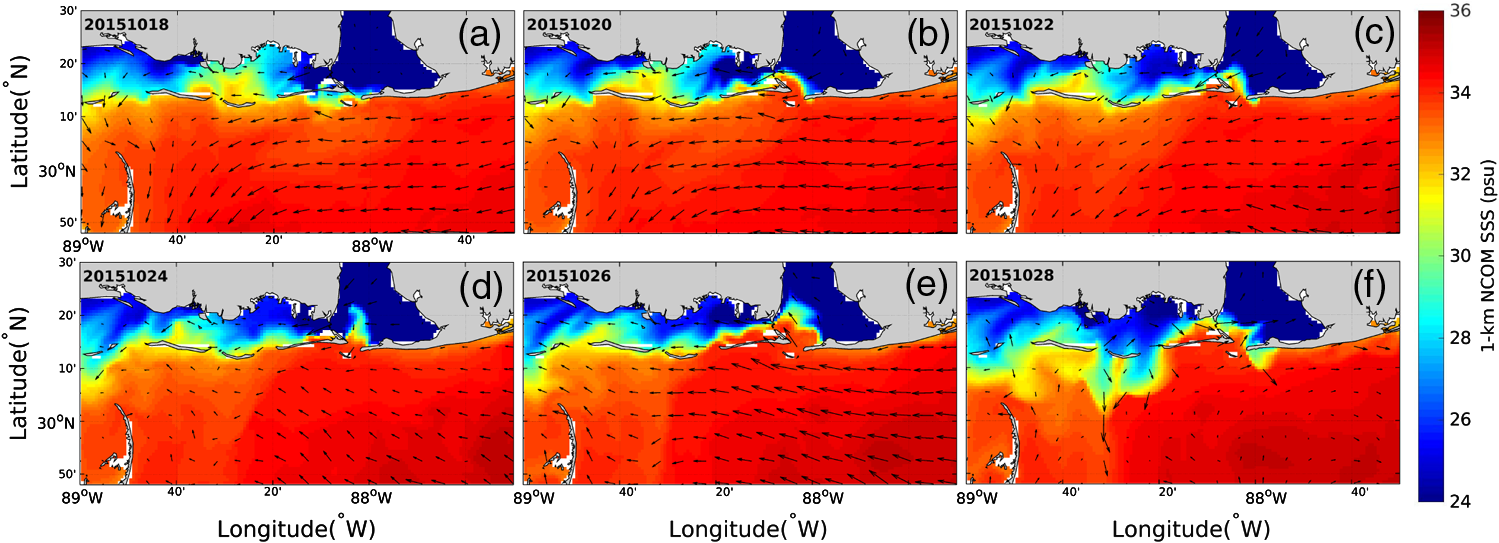 Velocity measurements (not shown here) at an inner-shelf mooring FOCAL station, located southwest of the Mobile Bay Main Pass [see Fig. 1(a) for location], showed that the currents were directed onshore, mainly in the NW direction from October 18 until the instrument was buried due to Patricia’s remnants on October 27, 2015. NCOM results in Fig. 3 show an inflow of high-salinity shelf waters via the Horn Island Pass before October 19, 2015 [Fig. 3(a)]. The model results show that higher salinity shelf waters reached the southern coastline of almost all barrier islands, entered the estuarine system mainly via the Mobile Bay Main Pass, mixed with estuarine waters, and then flowed west into the MSS via Grant Pass (Pass aux Herons) [Figs. 3(b)–3(e)]. Because of the wind reversal associated with Patricia’s remnants, estuarine waters were expected to be flushed out of the MSS and Mobile Bay as predicted by the model on October 28, 2015 [Fig. 3(f)]. Satellite imagery following passage of Patricia’s remnants (not shown here) also showed high-chlorophyll-a concentrations due to strong mixing, sediment resuspension, and increased biological activity in the freshwater plumes on the inner-shelf.51 Hovmoeller diagrams of NCOM SSS (0 to 2 m) along three chosen transects [Fig. 4(a); dashed lines] around the barrier island inlets are shown in Fig. 4. Figure 4(a) shows a zoomed-in map of the MSS barrier islands and passes. The southern-most transect is outside the Sound along 30.2°N and is aligned with Pelican, Petit Bois, and West Ship islands [Fig. 4(b)]. The salinity along the eastern side of the transect () shows salinities of inner-shelf waters above 32 psu, reaching and exceeding 34 psu. Lower salinity waters were predicted by the model to flush out of the Mobile Bay between October 11 and October 18, 2015, and later from October 27 to November 3, 2015, after the passage of Patricia’s remnants and a subsequent cold front on October 30, 2015. The flushing of lower salinity water from the Sound starting from October 27, 2015, was predicted to be stronger from the inlets around the Petit Bois Island most likely via both the Horn and Petit Bois passes. Lower salinity estuarine waters were predicted to continuously flush out of the Ship Island Pass during the entire month of October, while the intensity of flushing decreased between October 18 and 27, 2015. Fig. 4(a) Map of the MSS showing the major barrier islands and passes. NCOM predictions of sea surface salinity in between October 11 and November 11, 2015, through transects, (b) outside the Sound along 30.2°N(30°12’N), (c) along the passes at 30.24°N(30°14’24”N), and (d) inside the Sound along 30.3°N(30°18’N). Transect locations are shown in (a) as dashed lines.  Figure 4(c) shows the NCOM SSS through a transect north of the Mississippi barrier islands at 30.24°N crossing Dauphin Island and Fort Morgan, AL. This transect may be considered as the transition in between estuarine waters and shelf waters because it shows the signature of both lower salinity estuarine waters () and higher salinity shelf waters (). The model predicted strong northward transport of high-salinity waters through Mobile Bay Main Pass starting from October 18, 2015, and the inflow associated with this transport seems to prevent the flushing of Mobile Bay estuarine waters onto the shelf. The diagonal pattern of low-salinity waters from October 18 to October 27, 2015, shown in Fig. 4(c), suggests that the blockage of outflow at the Mobile Bay Main Pass and the strong easterly winds and currents caused the estuarine waters to be transported west from Mobile Bay toward the MSS. Therefore, it is likely that the low-salinity waters flushing out of the Horn Island and Petit Bois passes on October 27, 2015, could possibly be Mobile Bay estuarine waters transported westward during the 10-day period leading to the Patricia’s remnants passage over the study area. The last transect is inside the MSS and Mobile Bay at 30.3°N. Low-salinity () estuarine waters dominated throughout the period as shown in Fig. 4(d). The model predicted high-salinity shelf waters reaching this transect north of Mobile Bay Main Pass starting from October 19, 2015, with increasing intensity toward October 27, 2015. The salinity through this transect also showed an earlier high-salinity inflow via the Petit Bois Pass mixed with estuarine waters. These relatively high-salinity waters () were observed to be transported west between October 18 and October 27, 2015, possibly due to westward transport of Mobile Bay estuarine waters. 3.2.In situ Measurements in the Mississippi Sound and Mobile BayFigure 5 shows 40-h moving average filtered wind measurements at the OB buoy [Fig. 1(a); OB], water level, and salinity measurements (blue lines) at the Dauphin Island station [Fig. 1(a); DPHA] compared to the model predictions (red lines) during October 2015. Figure 5(a) and 5(b) show that the variability and magnitude of the East–West(u) and North–South(v) components of wind forcing from the COAMPS solution, used to force NCOM in October 2015, compare well with the measurements on the shelf at the OB buoy station southeast of the Mobile Bay Main Pass. The correlation coefficients between the u(E–W) and v(N–S) components of COAMPS wind variation and the measurements in October 2015 were and , respectively. Such high correlations indicate that the model forcing captured the wind variability on the shelf while the root mean squared error of modeled winds compared to the measurements is . Starting from October 16, 2015, the wind was predominantly southeasterly and easterly until a strong wind reversal happened due to Patricia’s remnants on October 27, 2015. The cross correlation of the model wind results with the measured winds showed that the u-component (E–W) of the model winds has a lag time of 2 h in regard to the field measurements, whereas the v-component (N–S) has no lag. Fig. 5Measurements (blue) versus NCOM model predictions (red) of (a) east–west wind speed at the OB buoy, (b) north–south wind speed at OB buoy, (c) water level at Dauphin Island station (DPHA) above Mean Lower Low Water (MLLW), and (d) salinity at Dauphin Island station (DPHA) in October 2015. Shown measurements and model results were 40-h moving average filtered. 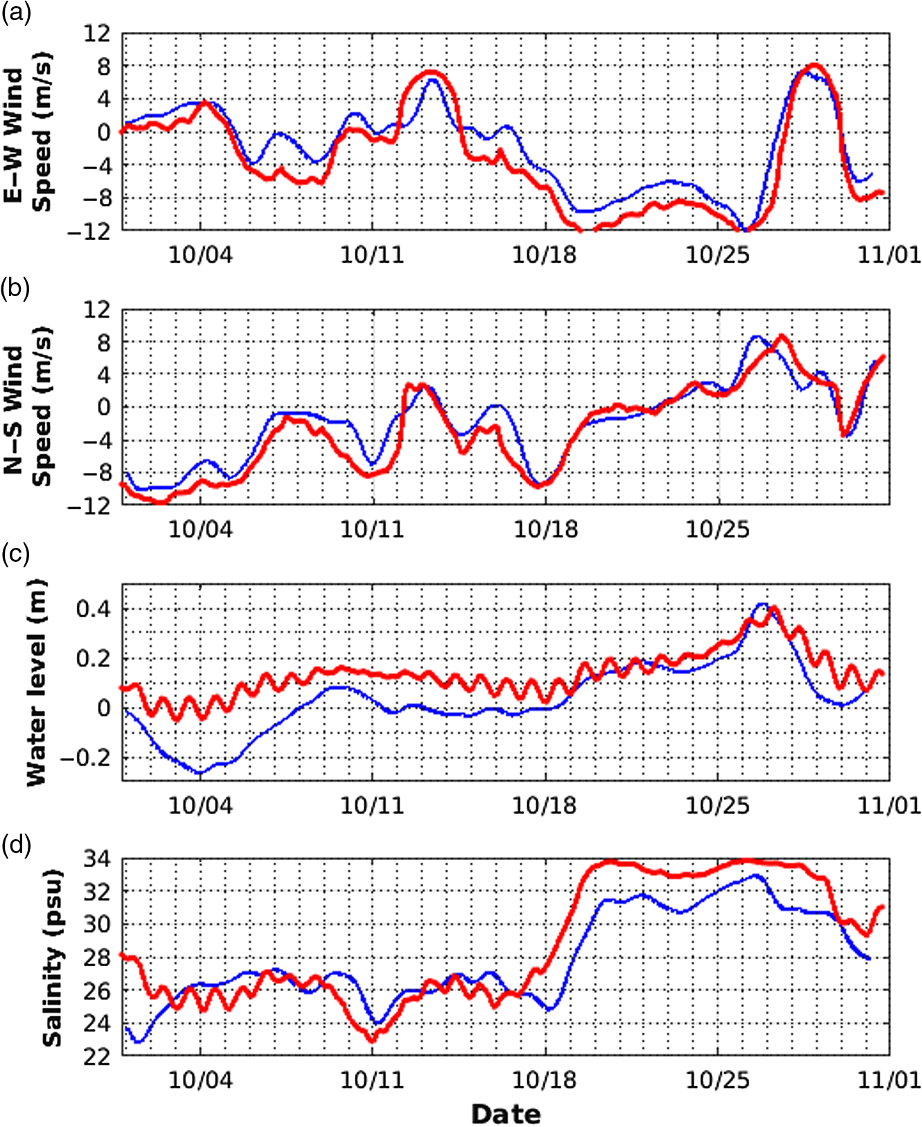 Figure 5(c) shows that the timing of model predictions for the water level peak and flushing was close to the measurements, with the peak magnitude matching the observed at the Dauphin Island station. The water surface elevation increased inside the MSS and Mobile Bay because of the trapping of estuarine waters combined with the surge. The salinity prediction of the model for October 2015 [Fig. 5(d)] was also in line with the measurements at Mobile Bay Main Pass (DPHA) with a correlation coefficient of for the month of October. Measurements showed that the salinity began to increase on October 18, 2015, and peaked at 33 psu during Patricia’s influence on October 27, 2015. Salinity then decreased with Patricia’s wind shift followed by several cold fronts to a value of 22 psu by early November 2015. The model salinity predictions were closer to the measurements between October 1 and 17 after which the model started consistently over-predicting the salinity. During the high-salinity event, the model consistently predicted between 1 and 2 psu above the measurements. Model-data comparison for winds indicate that the easterly winds are stronger in the model possibly causing a stronger inflow of estuarine waters into the estuarine system via Mobile Bay Main Pass as shown in Fig. 4(c). On October 27, 2015, the model salinity peak was 34 psu, compared to 33 psu measured at DPHA station. The root mean squared error for the modeled salinities at DPHA station compared to the measurements for the month of October 2015 was 1.77 psu while a comparison of modeled and measured salinities at the USM buoy at 20-m isobath [Fig. 1(a); USM] showed that the model results were within 0.5 psu of the measurements. Overall, the model predictions were in agreement with the measurements in capturing the trends during the time period of the inflow event in October 2015 validating the model’s capability to represent the estuarine-shelf exchange at the barrier island inlets. The discrepancies between model and measurements for high-salinity values during the inflow event may be because the ambient salinity on the shelf or in the estuaries may be higher in the model causing higher salinities predicted by the model during the inflow event. In addition, the horizontal diffusion or the vertical mixing of the 1-km model at these small scales for the shallow waters of the nGoM may result in such discrepancies between the model and the measurements at the mouth of Mobile Bay. Surface salinity measurements at the USM buoy (results not shown here), located at the 20-m isobath [Fig. 1(a); USM], showed the salinity at the inner-shelf exceeded 30 psu in July 2015 and stayed over 30 psu until the end of the calendar year. Moreover, the USM buoy showed the salinity in October remained over 33.5 psu for the majority of October 2015 until a 2-psu drop from 34.5 to 32.5 psu due to Patricia’s remnants moving over the area. Figure 6 shows salinity measurements (blue) recorded at 30-min (DPHA, CRTA) or 6-min (M14) frequency at stations in the study area along with the 36-h moving averaged salinity variations (red) to filter out the tidal fluctuations. Figure 6(a) shows salinity at the Dauphin Island station [Fig. 1(a); DPHA] recorded every 30 min (blue) between 2011 and 2015, and Fig. 6(b) shows the salinity for 2015 only. Salinity increased during the spring and summer for all years and peaked during the fall months. It is seen that the salinity rarely exceeded 30 psu between 2011 and 2015. In fact, salinity only exceeded 30 psu for a combined duration of less than 12, 9, 6, 3, and 23 days during 2011, 2012, 2013, 2014, and 2015, respectively. Therefore, we choose 30 psu as a high-salinity threshold at this station and north of the barrier islands. Salinity exceeded this threshold at DPHA only episodically and for short intervals. In fact, fall 2015 was the only period when the salinity exceeded and persisted over 30 psu for an extended period of time (7.5 days) and over 29 psu for 11 straight days. Figure 6(b) shows that salinity records at Dauphin Island station, DPHA, remained over 30 psu for most of the second half of October. A similar persistent salinity increase was also observed in other stations in the MSS. Fig. 6Salinity measurements (raw data in blue and 36-h filtered data in red) at (a) DPHA station from 2013 to 2015 and a subset for only 2015 data for stations at: (b) DPHA, (c) CRTA, and (d) M14.  The salinity measurement at CRTA station [Fig. 1(a)] on the eastern side of the MSS close to Mobile Bay is shown in Fig. 6(c). Since this station is north of the barrier islands and inside the MSS, the peak salinity was lower than the DPHA station due to the proximity to low-salinity freshwater sources and mixing inside the estuarine system. However, while the salinity at this station reached 25 psu episodically, it exceeded 25 psu in October 2015, and similar to DPHA, it stayed over this value for more than a week. Figure 6(d) shows the salinity measurements at MDMR/USGS station M14 which is on the western end of the MSS [Fig. 1(a); M14]. The salinity exceeded 30 psu in mid-October and stayed above 30 psu for the same late-October duration shown in the other stations. The fact that similar salinity fluctuations were seen not only at the DPHA but also at CRTA and M14 at both ends of the MSS indicates that the inflow of saline waters was a system-wide event impacting the entire MSS. Since high-salinity events in the MSS are indicative of intrusions of high-salinity shelf water, these events have important implications for potential transport of larvae, pollutants, and toxic algae into the MSS. An important question then is to understand whether the high-salinity signal observed in October 2015 is atypical or not. To do that, the October 2015 event was compared with October conditions in other years. An anomaly study on salinity measurements was conducted for these purposes. A 9-year monthly climatology of salinity values from 2007 to 2015 was generated using salinity from near-bottom temperature and conductivity measurements at MDMR/USGS stations. Monthly mean salinities were calculated for the entire time series at each station. Monthly anomalies were calculated as the difference between the monthly climatology [, average from 2007 to 2015] and the monthly mean value of each year (). Figure 7 shows the salinity anomalies for the last 5 years (2011 to 2015) of the 9-year period, during which interannual fluctuations were apparent. Elevated salinity shown as positive salinity anomaly peaks in late summer and fall months (August to October) in 2014 and 2015 at all stations, and early summer months (May to July) in 2011 and 2012 at most stations. The highest positive salinity anomaly was seen in October 2015 (shown in red) at all MDMR/USGS stations across the MSS. Monthly anomalies for temperature and water surface elevation measurements at MDMR stations (not shown here) were also calculated. Temperature anomalies showed no significant difference between years at all stations. October 2015 had one of the highest sea surface elevation anomalies (up to 50 cm higher water level) during the 2011 to 2015 time frame due to the passage of Patricia’s remnants. Figure 8(a) shows the October in situ mean salinities and variability from 2007 to 2015 at the MDMR/USGS stations and the NOAA/NDBC stations in the study area. October mean salinities were the highest in 2015 at all stations. This indicates that October 2015 had more saline offshore water inflow into the MSS and Mobile Bay and toward the station locations. The highest salinities of October 2015 were measured at the MSS stations; M2, M6, M7, M14, DPHA, and PPTA. Stations M2, M6, M7, and M14 were either near the barrier island inlets (M6, M14) or relatively away from the coastline and freshwater sources (M2, M7). Fig. 8(a) October mean salinities from 2007 to 2015 at the MDMR/USGS and NOAA/NDBC stations. Number of days when the October mean salinities exceed (b) 30 psu (c) 26 psu at all the stations (gray areas indicate no data). (d) Study area showing station locations. 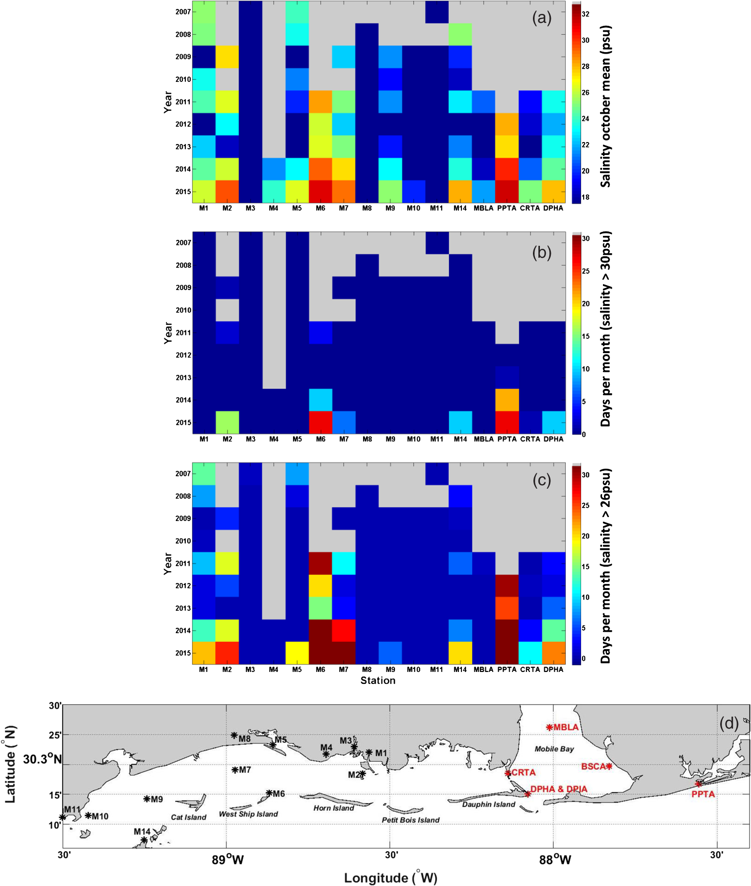 The DPHA station at Dauphin Island is exposed to saline offshore waters via the exchange through the Mobile Bay Main Pass, while PPTA at Perdido Pass is already located at the Gulf of Mexico coastline directly exposed to the inner-shelf waters. In addition to examining monthly mean salinity, it is also important to know for how long salinity exceeded a certain threshold. Figure 8(b) shows the number of days in October for which salinity exceeded 30 psu. It is clear that 2015 had the most number of days, especially at those stations with the highest monthly mean salinities mentioned above. For M6 and PPTA, the salinity exceeded 30 psu for over 25 days in October 2015, followed by M2 where the salinity exceeded the 30 psu threshold for at least 15 days. At M7, M14, and DPHA, measured salinity exceeded 30 psu for at least 10 days in October 2015 and did not exceed this threshold in any of the other years with available salinity measurements. Some stations, e.g., M3, M4, M8, M10, M11, and MBLA, were never exposed to salinities above 30 psu due to proximity to freshwater sources, therefore, a lower salinity threshold of 26 psu was also used at all stations between 2007 and 2015. Figure 8(c) shows that the salinity values exceeded 26 psu at least at one station each year, but the exceedance frequency was the highest in 2015. Measured salinity exceeded the 26-psu threshold more frequently in October months of 2014 and 2015. It was found that the salinity exceeded this value for most if not all days in the month of October at the only open water station PPTA. The exceedance ratio was also high at M6 and M7, followed by M2, DPHA, and M14. While the salinity never exceeded 30 psu at M1 and M5, it exceeded 26 psu for more than 2 weeks at M1 and M5. Figure 8 highlights that October 2015 was different from earlier years and that the salinity in all these coastal stations were higher than usual within the 9-year time period of 2007 to 2015. 3.3.Ocean Color DataThe analysis using the NCOM salinity and the salinity exceedance and anomaly analysis on the in situ measurements demonstrated that October 2015 had a high-salinity event at multiple stations across the system from Mobile Bay to western MSS. Satellite ocean color chlorophyll-a imagery was used to determine the corresponding surface, or more precisely over the first optical depth, biological response associated with the anomalous surface salinity conditions over the broader region. MODIS-Aqua October monthly chlorophyll-a anomaly fields were calculated for the Mississippi Bight from 2003 to 2015 and shown in Fig. 9. The October 2015 monthly chlorophyll-a anomaly has a negative anomaly (less chlorophyll-a than the monthly climatology) across the entire Mississippi Bight except very near the Mississippi river outlets in the Bird Foot Delta. The only other year with negative chlorophyll-a anomaly to such a great extent was 2003. The other years at least have a positive anomaly either outside the MSS on the shelf or inside the MSS. The reason for most years to have positive chlorophyll-a anomaly either inside the MSS or just south of the barrier islands is probably high chlorophyll-a associated with freshwater sources inside the MSS and plume waters coming out of the estuarine system. Figure 10 shows the October monthly chlorophyll-a anomaly of each year along transects (Fig. 1; red lines) inside the MSS [Fig. 10(a)] north of the barrier islands and outside the MSS [Fig. 10(b)]. Ocean color data clearly shows that October 2015 has the largest negative chlorophyll-a anomaly both inside and outside the MSS. It is important to notice that 2015 is not the only year with such high-negative chlorophyll-a anomaly ( to ) at both transects. October 2003 had a similar chlorophyll-a anomaly. Fig. 9October monthly mean MODIS-Aqua chlorophyll-a anomaly in the Mississippi Bight from 2003 to 2015.  Fig. 10October monthly mean MODIS-Aqua chlorophyll-a anomaly () from 2003 to 2015 along a transect (a) inside the MSS and (b) outside the MSS. Transect locations plotted in Fig. 1(a) as dotted red lines.  While chlorophyll-a anomaly is generally positive inside the MSS due to freshwater dominance that brings sediment and nutrients, it is generally negative outside the MSS due to offshore water dominance. October 2007 and 2013 had low-chlorophyll-a anomalies ( to ) inside the MSS similar to October 2015, but not necessarily as negative a chlorophyll-a anomaly as October 2015 outside the MSS. So, the negative chlorophyll-a anomaly outside the MSS may be attributed to the fact that the shelf was covered by low-chlorophyll-a/less turbid offshore saline waters outside the MSS in October 2015 and the estuarine low-salinity high chlorophyll-a, and turbid waters were not flushed out of the MSS preventing the formation of high-chlorophyll-a plumes during most of the month. An ANOVA was performed on the October monthly anomaly values to see the difference in chlorophyll-a anomaly by year followed by a multiple comparison test on the monthly mean chlorophyll-a anomaly to determine which years had a chlorophyll-a anomaly distribution either similar to or significantly different from October 2015 inside and outside the MSS [see Fig. 15 in the Appendix]. Outside the MSS, the October 2003 anomaly was the only one similar to October 2015 and all the other years were significantly different. Inside the MSS, the multiple year comparison showed that October 2003 and October 2007 were similar to October 2015 with low chlorophyll-a. The other 10 years were found to be significantly different and have higher chlorophyll-a than 2015, but the October 2013 results had the closest anomaly means [Fig. 15 in the Appendix) and was similar to October 2015 in transect lines both inside and just outside the MSS. 3.4.Meteorological and Hydrological DataIt is important to understand the forcing mechanisms that generated the high-positive salinity anomaly along with the low-negative chlorophyll-a anomaly in October 2015. For this reason, the meteorological data (i.e., wind, water level) and hydrological data (i.e., discharge from freshwater sources into the MSS and Mobile Bay) were analyzed to understand the balance between high-salinity/low-chlorophyll-a offshore waters and the low-salinity/high-chlorophyll-a freshwater sources. The role of wind forcing was assessed using a correlation analysis between the wind measured at the OB Buoy [Fig. 1(a); OB] and the adjusted water level (i.e., inverse barometer effects removed) and salinity data at the Dauphin Island station [Fig. 1(a); DPHA]. The component of the wind forcing with the maximum correlation was determined by calculating a lagged correlation between wind vector component contribution at 5-deg intervals and the scalar parameter of interest (water level or salinity) during the month of October. The highest correlations between the wind component and water level were along the orientation of 290 to 330 deg/110 to 150 deg (i.e., NW/SE axis) with -values of 0.90 to 0.93 with lags of 12 to 23 h. Similarly, the highest correlations between the wind component and salinity were along the orientation of 315 to 350 deg/135 to 170 deg (i.e., NNW/SSE axis) with -values of 0.80 to 0.92 corresponding to lags of 0 to 2 h. These results are consistent with the combined effects of coastal Ekman circulation driving coastal set-up and set-down via along-shelf wind forcing, as well as direct wind forcing from the N/S component in the shallower coastal areas where the Ekman boundary layers would be expected to overlap (i.e., water is being directly pushed onshore contributing to the coastal set-up or set-down). The wind-driven changes in coastal water level result in estuarine-shelf exchange that alter the estuarine salinity as observed. Salinity is somewhat more sensitive to the N/S component as indicated by the more NNW/SSE orientation and shorter lag time (i.e., direct wind response would be expected to be faster than the local Coriolis timescale). This correlation analysis shows that the wind forcing was the primary driver of the low-frequency salinity variability during this period and that wind generally from the southeast quadrant is favorable for high-salinity intrusion events. The correlation analysis (above) showed positive correlation between wind and salinity in the 40- to 215-deg interval with decreasing correlation for directions larger than 180 deg. Given that southerly to easterly winds could drive salinity intrusions, the wind from the 45- to 180-deg direction is considered favorable for forcing the transport of saline offshore waters toward all the barrier islands around the MSS including the N–S oriented Chandeleur Islands. In particular, 13 years (2003 to 2015) of wind data for October at the Dauphin Island station (Fig. 1; DPIA) were analyzed. An important factor to consider is the wind persistence for a nonstop consecutive time. Consecutive winds in certain directions will force saline offshore waters toward the MSS and Mobile Bay, as well as prevent estuarine waters from flowing out of the MSS and Mobile Bay. We found that the number of consecutive hours in October since 2003 with the winds within the 45- to 180-deg interval was the highest in 2015 with 204 consecutive hours. This is approximately an 8.5-day period between October 19 and 27, 2015. October 2013 winds follow with 143 consecutive hours, October 2004 with 132, and October 2007 with 122 consecutive hours of wind within the favorable 45 to 180 deg interval. The October monthly chlorophyll-a anomaly for 2003 and 2007 was statistically similar to October 2015, however, the October 2013 salinity anomaly was not as high as that of 2015. Unfortunately, there were no salinity measurements available from 2007 to compare. It is not only the persistence of wind from favorable directions, but also the strength of the wind that will impact the intensity of forcing. Therefore, wind roses were created for those periods when the wind at the DPIA station was consecutively within the 45- to 180-deg interval to visualize the directional spread within the interval along with the wind speed as shown in Fig. 11. The time period in which the wind was persistently within the 45- to 180-deg interval is shown below the wind rose of each year. The wind speed exceeded only in October 2015 (Fig. 11; at the bottom), 2004, and 2006; and for all these years, wind was from E-SE for more than 50% of the favorable wind window. While the wind speed was high in 2006, the number of consecutive hours was lower (64 h). On the other hand, 2004 winds were strong, but Figs. 9 and 10 indicate that this was a high-chlorophyll-a year possibly due to high-freshwater discharge both from the Mississippi River onto the shelf and/or from other sources into the MSS. Fig. 11October wind roses from 2003 to 2015 during the time windows when the wind was uninterruptedly from the [45-180°] direction interval.  Figure 12(a) shows the river discharges measured at USGS stream gauges at Pearl, Pascagoula, Alabama, and Mobile Rivers (see Table 1 for station locations). In 2015, the river discharge was lowest in August, September, and November at all river systems in the area. Both the Pearl and Mobile Rivers are good indicators of the variability of freshwater input intensity in our region because of their discharges into the MSS and Mobile River, respectively. Therefore, the October discharges from 2007 to 2015 for those two rivers were analyzed in Figs. 12(b)–12(i). October 2009 was not shown in Fig. 12 due to the extremely high-discharge offsetting the -axis. Measurements from the Pascagoula and Alabama rivers were not shown in Fig. 12 due to their similarity to the Pearl and Mobile Rivers’ discharges, respectively. Fig. 12(a) Calendar year 2015 discharge measurements at Pearl, Pascagoula, Alabama, and Mobile Rivers. (b)–(i) October discharge measurements at Pearl River (blue) and Mobile River (green) from 2007 to 2015. October 2009 is not shown due to extremely high-discharge offsetting the -axis.  The discharge at Pearl River was seasonally low and around for almost all years and was generally less than for the Mobile River. The Mobile River showed higher fluctuations within October 2015, however, discharge variations were similar for both rivers. At Pearl River, October 2007 and 2010 had the lowest discharges, along with 2015, until the discharge peaks after passage of cyclone Patricia’s remnants in late October 2015. At Mobile River, the discharge was very low between October 19 and 26, 2015, but the lowest October discharge year was 2010, followed by 2011. While high-freshwater input into the Mobile Bay and MSS is expected to decrease the likelihood of having elevated salinities inside the estuarine system, similarity in the intensity of discharge for all years implies that the low rainfall and low discharge in the area were not a significant contributing mechanism for the increased salinities inside the MSS and Mobile Bay while the wind over the area is the primary driver for the inflow event. 4.ConclusionThis study combined model forecast products, in situ measurements, and satellite imagery data to study an episodic strong and persistent inflow and intrusion of high-salinity offshore Gulf of Mexico waters into the MSS and Mobile Bay estuarine systems. In situ measurements showed elevated salinity measurements at coastal stations for an extended period (from October 18 to October 27, 2015) before Patricia’s remnants passed. Monthly anomalies of salinity, temperature, and water level were calculated from 2007 to 2015 in the Sound. All stations inside the MSS had the highest positive salinity anomalies during October 2015 suggesting an excessive influx of saline shelf waters into the Sound. Model predictions of surface salinity and current fields showed an inflow of shelf waters into the estuarine system mainly via the Mobile Bay Main Pass due to strong easterly/southeasterly currents on the shelf. Patricia’s remnants in late October further enhanced the positive salinity anomaly. This strong inflow into Mobile Bay possibly prevented the flushing until the passage of Patricia’s remnants and several cold fronts. MODIS-Aqua monthly chlorophyll-a anomalies were calculated from 2003 to 2015 using monthly means and climatology to define the biological response to the physical processes before the passage of Patricia’s remnants. The October 2015 chlorophyll-a anomaly had the lowest (negative) anomaly both inside the MSS and outside on the Mississippi Bight shelf indicating a reduced biological activity in near-surface waters. A multicomparison test of all the October chlorophyll-a monthly anomalies revealed that all years except 2003 were significantly different from 2015 for both inside and outside the MSS. The chlorophyll-a anomaly for October 2007 showed a similar chlorophyll anomaly to 2003 and 2015 inside the MSS. Unfortunately, the limited salinity dataset for 2007 does not allow us to make a definitive conclusion; however, the low-chlorophyll-a anomaly could be due to low discharge and weaker westward transport (NCOM model current data for 2007 not shown). The anomaly analysis on both in situ measurements and satellite imagery combined with the model forecast fields indicated that the high-salinity offshore waters were brought onto the entire Mississippi Bight shelf and the currents transported them into the estuaries where both low-salinity estuarine waters and high-salinity shelf waters were transported west due to strong easterly currents. A salinity exceedance analysis at all stations showed that October 2015 had the highest salinity records at many stations across the MSS, showing that this episodic event was a system-wide event. An analysis of the hydrology and meteorology of the study area showed that the river flow was seasonally low during the time of the shelf water intrusion event before it peaked due to the heavy precipitation of Patricia’s remnants and subsequent cold fronts. The inflow event preceding the passage of cyclone Patricia’s remnants followed by Patricia’s wind shift allowed the flushing of the estuarine waters onto the shelf creating plumes on the inner-shelf and mid-shelf accompanied with strong mixing and resuspension due to the storm. The highest correlation between wind and salinity was found for the wind from the [45-180]° direction interval. The correlation between wind and water level was also high in the interval showing that the coastal set-up and the rise in October 2015 were mainly due to onshore shelf wind forcing. Easterly, southeasterly, and southerly winds were persistent in October 2015 during the 8-day period leading to this wind shift. An analysis on the uninterrupted wind from the [45-180]° direction for all years showed that October 2015 had the longest duration for this wind interval, which is possibly favorable to create currents that will allow the influx of shelf waters into the MSS and Mobile Bay and to block estuarine waters in the Sound and Bay. After the DWH oil spill event, special attention has been directed to the circulation and dynamics near susceptible coastal ecosystems such as the estuaries within the Mississippi Bight. Their valuable fisheries and nursery habitats could be negatively impacted or even collapse in the case of toxic oil/dispersant or harmful algal blooms events. The MSS and Mobile Bay are river discharge dominated systems, although the exchange with saline Mississippi Bight Shelf waters is tide-dominated and occur frequently in short-time episodic events. Results show that the MSS and Mobile Bay are not only limited to short-time episodic events (hours to a few days), but strong and persistent () inflow of saline Mississippi Bight shelf waters occur. October seems to be a favorable month for extended intrusion of offshore waters types of events, so special attention needs to be considered for an oil spill during this time frame. The results conclude that the MSS was exposed to elevated salinities for over 10 days due to inflow and intrusion of shelf waters during this October 2015 event, which, if this happened concurrently with an oil spill could be detrimental to the coastal habitats and local fisheries. AppendicesAppendixQuality controlled MODIS-Aqua Level-3 SMI chlorophyll-a monthly means and climatology at 4-km spatial resolution were downloaded from the NASA-Ocean Biology Processing Group website.43 Figure 13 shows the MODIS-Aqua October chlorophyll-a monthly mean fields for the study area from 2003 to 2015 and Fig. 14 shows the 13-year MODIS-Aqua October monthly mean climatology field for the entire time period. The results for the October monthly mean chlorophyll-a anomaly fields calculated from the monthly mean and the climatology fields were shown in Fig. 9. Fig. 14MODIS-Aqua October chlorophyll-a climatology in the Mississippi Bight derived from October monthly means from 2003 to 2015. 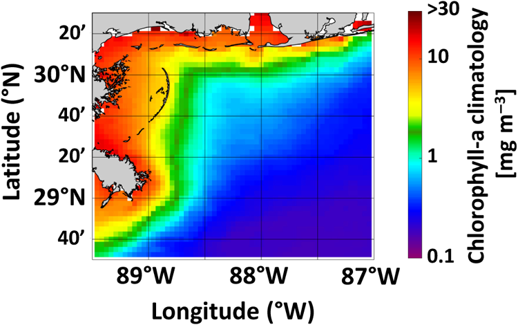 An ANOVA was performed on the October monthly anomalies inside and outside the Sound shown in Figs. 9 and 10. A multiple comparison test was conducted on the statistics of the ANOVA results to find out which years had significantly different chlorophyll-a anomalies than that of October 2015 inside and outside the MSS. ANOVA results showed that the p-value was very small () both inside and outside the Sound indicating that differences between means were significant and October 2015 had a significantly different chlorophyll-a distribution than other years. Figure 15 shows the results of the multiple comparison test. AcknowledgmentsThis research was made possible by a grant from The Gulf of Mexico Research Initiative (GoMRI). The CONsortium for oil spill exposure pathways in COastal River Dominated Ecosystems (CONCORDE) program contributed to this work. We would like to thank other participants of the CONCORDE consortium for their scientific discussions in the valuable publication workshops of CONCORDE. NCOM model data are publicly available and accessible through the Gulf of Mexico Research Initiative Information and Data Cooperative (GRIIDC) at https://data.gulfresearchinitiative.org (DOI: 10.7266/N7HX1B37). Aspects of the data were collected with the help of the Tech Support Group at the Dauphin Island Sea Lab, including G. Lockridge, Y. Hintz, and L. Linn, and the Alabama Realtime Coastal Ocean Observing System program manager, R. Collini (data available at www.mymobile.com). We thank the NASA Goddard Space Flight Center, Ocean Ecology Laboratory, Ocean Biology Processing Group for the Moderate-Resolution Imaging Spectroradiometer (MODIS)-Aqua Chlorophyll Data; 2014 Reprocessing. NASA OB.DAAC, Greenbelt, Maryland (DOI: http://dx.doi.org/10.5067/AQUA/MODIS/L3M/CHL/2014). References“Environmental response management application (2017) web application,”
(2017) http://response.restoration.noaa.gov/erma/ January 2017). Google Scholar
T. B. Kimberlain, E. S. Blake and J. P. Cangialosi,
“Hurricane Patricia (EP202015) 20– 24 October 2015,”
National Hurricane Center Tropical Cyclone Report, National Hurricane Center, Miami, Florida
(2016). Google Scholar
E. K. Chesney, D. M. Baltz and R. G. Thomas,
“Louisiana estuarine and coastal fisheries and habitats: perspectives from a fish’s eye view,”
Ecol. Appl., 10 350
–366
(2000). http://dx.doi.org/10.1890/1051-0761(2000)010[0350:LEACFA]2.0.CO;2 ECAPE7 1051-0761 Google Scholar
R. J. Zimmerman, T. J. Minello, L. P. Rozas,
“Salt marsh linkages to productivity of penaeid shrimps and blue crabs in the northern Gulf of Mexico,”
Concepts and Controversies in Tidal Marsh Ecology, 293
–314 Springer, Netherlands
(2000). Google Scholar
I. A. Mendelssohn et al.,
“Oil impacts on coastal wetlands: implications for the Mississippi River delta ecosystem after the Deepwater Horizon oil spill,”
BioScience, 62
(6), 562
–574
(2012). http://dx.doi.org/10.1525/bio.2012.62.6.7 BISNAS 0006-3568 Google Scholar
M. Love et al., The Gulf of Mexico Ecosystem: A Coastal and Marine Atlas, Ocean Conservancy, Gulf Restoration Center, New Orleans, Louisiana
(2013). Google Scholar
II E. C. Blancher et al.,
“Simulation of exposure, bioaccumulation, toxicity and estimated productivity losses from the Deepwater Horizon oil release in the Mississippi-Alabama nearshore marine environment,”
in SETAC European Conf.,
(2016). Google Scholar
W. M. Graham et al.,
“Oil carbon entered the coastal planktonic food web during the Deepwater Horizon oil spill,”
Environ. Res. Lett., 5 045301
(2010). http://dx.doi.org/10.1088/1748-9326/5/4/045301 Google Scholar
B. Graham et al.,
“Deep water–the gulf oil disaster and the future of offshore drilling,”
Report to President, National Commission on the BP Deepwater Horizon Oil Spill and Offshore Drilling, 129
–170 U.S. Government Publishing Office, Washington, DC
(2011). Google Scholar
Q. Dortch, T. Peterson and R. E. Turner,
“Algal bloom resulting from the opening of the Bonnet Carré Spillway in 1997,”
in Basics of the Basin Research Symp.,
(1998). Google Scholar
A. F. Maier Brown et al.,
“Effect of salinity on the distribution, growth, and toxicity of Karenia spp,”
Harmful Algae, 5 199
–212
(2006). http://dx.doi.org/10.1016/j.hal.2005.07.004 HALNE7 Google Scholar
C. K. Eleuterius,
“Classification of Mississippi Sound as to estuary hydrological type,”
Gulf Res. Rep., 6 185
–187
(1978). http://dx.doi.org/10.18785/grr.0602.12 GURRA4 Google Scholar
R. P. Stumpf, G. Gelfenbaum and J. R. Pennock,
“Wind and tidal forcing of a buoyant plume, Mobile Bay, Alabama,”
Cont. Shelf Res., 13 1281
–1301
(1993). http://dx.doi.org/10.1016/0278-4343(93)90053-Z CSHRDZ 0278-4343 Google Scholar
J. L. Cowan et al.,
“Seasonal and interannual patterns of sediment-water nutrient and oxygen fluxes in Mobile Bay, Alabama (USA): regulating factors and ecological significance,”
Mar. Ecol. Prog. Ser., 141 229
–245
(1996). http://dx.doi.org/10.3354/meps141229 MESEDT 0171-8630 Google Scholar
S. Vinogradov et al.,
“Temperature and salinity variability in the Mississippi Bight,”
Mar. Technol. Soc. J., 38
(1), 52
–60
(2004). http://dx.doi.org/10.4031/002533204787522433 MTSJBB 0025-3324 Google Scholar
N. Vinogradova et al.,
“Evaluation of the Northern Gulf of Mexico littoral initiative (NGLI) model based on the observed temperature and salinity in the Mississippi bight shelf,”
Mar. Technol. Soc. J., 39
(2), 25
–38
(2005). http://dx.doi.org/10.4031/002533205787443999 Google Scholar
Jr. S. P. Orlando et al., Salinity Characteristics of Gulf of Mexico Estuaries, 209 National Oceanic and Atmospheric Administration, Office of Ocean Resources Conservation and Assessment, Silver Spring, Maryland
(1993). Google Scholar
B. Dzwonkowski et al.,
“Hydrographic variability on a coastal shelf directly influenced by estuarine outflow,”
Cont. Shelf Res., 31 939
–950
(2011). http://dx.doi.org/10.1016/j.csr.2011.03.001 CSHRDZ 0278-4343 Google Scholar
R. He and R. H. Weisberg,
“West Florida shelf circulation and temperature budget for the 1998 fall transition,”
Cont. Shelf Res., 23 777
–800
(2003). http://dx.doi.org/10.1016/S0278-4343(03)00028-1 CSHRDZ 0278-4343 Google Scholar
B. Dzwonkowski and K. Park,
“Influence of wind stress and discharge on the mean and seasonal currents on the Alabama shelf of the northeastern Gulf of Mexico,”
J. Geophys. Res., 115
(C12052), 1
–11
(2010). http://dx.doi.org/10.1029/2010JC006449 Google Scholar
P. Chigbu, S. Gordon and T. Strange,
“Influence of inter-annual variations in climatic factors on fecal coliform levels in Mississippi Sound,”
Water Res., 38 4341
–4352
(2004). http://dx.doi.org/10.1016/j.watres.2004.08.019 WATRAG 0043-1354 Google Scholar
D. R. Johnson, H. M. Perry and W. M. Graham,
“Using nowcast model currents to explore transport of non-indigenous jellyfish into the Gulf of Mexico,”
Mar. Ecol. Prog. Ser., 305 139
–146
(2005). http://dx.doi.org/10.3354/meps305139 MESEDT 0171-8630 Google Scholar
T. R. Keen,
“Waves and currents during a winter cold front in the Mississippi bight, Gulf of Mexico: implications for barrier island erosion,”
J. Coastal Res., 18
(4), 622
–636
(2002). JCRSEK 0749-0208 Google Scholar
B. Kjerfve,
“Analysis and synthesis of oceanographic conditions in Mississippi Sound, April–October 1980,”
Mobile, Alabama
(1983). Google Scholar
B. Dzwonkowski, K. Park and R. Collini,
“The coupled estuarine-shelf response of a river-dominated system during the transition from low to high discharge,”
J. Geophys. Res. Oceans, 120 6145
–6163
(2015). http://dx.doi.org/10.1002/2015JC010714 JGRCEY 0148-0227 Google Scholar
B. Dzwonkowski et al.,
“Spatial variability in the spring velocity structure on a river-influenced inner shelf in coastal Alabama,”
Cont. Shelf Res., 74 25
–34
(2014). http://dx.doi.org/10.1016/j.csr.2013.12.005 CSHRDZ 0278-4343 Google Scholar
J. C. Dietrich et al.,
“Surface trajectories of oil transport along the Northern Coastline of the Gulf of Mexico,”
Cont. Shelf Res., 41 17
–47
(2012). http://dx.doi.org/10.1016/j.csr.2012.03.015 CSHRDZ 0278-4343 Google Scholar
E. D. Zaron et al.,
“Initial evaluations of a U.S. Navy rapidly relocatable Gulf of Mexico/Caribbean ocean forecast system in the context of the Deepwater Horizon oil spill disaster,”
Front. Earth Sci., 9 25
–34
(2015). http://dx.doi.org/10.1007/s11707-014-0508-x Google Scholar
R. Arnone et al.,
“Surface biomass flux across the coastal Mississippi shelf,”
Proc. SPIE, 9827 98270Z
(2016). http://dx.doi.org/10.1117/12.2240874 PSISDG 0277-786X Google Scholar
C.-K. Kim and K. Park,
“A modeling study of water and salt exchange for a micro-tidal, stratified northern Gulf of Mexico estuary,”
J. Mar. Syst., 96–97 103
–115
(2012). http://dx.doi.org/10.1016/j.jmarsys.2012.02.008 JMASE5 0924-7963 Google Scholar
B. M. Webb and C. Marr,
“Spatial variability of hydrodynamic timescales in a broad and shallow estuary: Mobile Bay, Alabama,”
J. Coastal Res., 32
(6), 1374
–1388
(2016). http://dx.doi.org/10.2112/JCOASTRES-D-15-00181.1 JCRSEK 0749-0208 Google Scholar
H. E. Seim, B. Kjerfveb and J. E. Sneed,
“Tides of Mississippi Sound and the adjacent continental shelf,”
Estuarine Coastal Shelf Sci., 25 143
–156
(1987). http://dx.doi.org/10.1016/0272-7714(87)90118-1 ECSSD3 0272-7714 Google Scholar
C. K. Eleuterius,
“Geographical definition of Mississippi Sound,”
Gulf Res. Rep., 6 179
–181
(1978). http://dx.doi.org/10.18785/grr.0602.10 GURRA4 Google Scholar
G. B. Austin,
“On the circulation and tidal flushing of Mobile Bay, Alabama,”
(1953). http://hdl.handle.net/1969.1/ETD-TAMU-1953-THESIS-A935 Google Scholar
C. N. Barron et al.,
“Sea surface height predictions from the global navy coastal ocean model (NCOM) during 1998-2001,”
J. Atmos. Oceanic Technol., 21 1876
–1893
(2004). http://dx.doi.org/10.1175/JTECH-1680.1 JAOTES 0739-0572 Google Scholar
C. N. Barron et al.,
“Formulation, implementation and examination of vertical coordinate choices in the global navy coastal ocean model (NCOM),”
Ocean Modell., 11
(3–4), 347
–375
(2006). http://dx.doi.org/10.1016/j.ocemod.2005.01.004 1463-5003 Google Scholar
A. B. Kara et al.,
“Validation of interannual simulations from the 1/8° global navy coastal ocean model (NCOM),”
Ocean Modell., 11
(3–4), 376
–398
(2006). https://doi.org/10.1016/j.ocemod.2005.01.003 1463-5003 Google Scholar
R. M. Hodur,
“The Naval Research Laboratory’s Coupled Ocean/Atmosphere Mesoscale Predication System (COAMPS),”
Mon. Weather Rev., 125 1414
–1430
(1997). http://dx.doi.org/10.1175/1520-0493(1997)125<1414:TNRLSC>2.0.CO;2 MWREAB 0027-0644 Google Scholar
S. Chen et al.,
“COAMPSTM version 3 model description—general theory and equations,”
141
(2003). Google Scholar
R. A. Allard et al.,
“Validation test report for the coupled ocean atmospheric mesoscale prediction system (COAMPS) version 5,”
172
(2010) http://www7320.nrlssc.navy.mil/pubs/2010/allard2-2010.pdf Google Scholar
G. D. Egbert, A. F. Bennett and M.G.G. Foreman,
“Topex/Poseidon tides estimated using a global inverse model,”
J. Geophys. Res., 99 24821
–24852
(1994). http://dx.doi.org/10.1029/94JC01894 JGREA2 0148-0227 Google Scholar
G. D. Egbert and S. Y. Erofeeva,
“Efficient inverse modeling of barotropic ocean tides,”
J. Atmos. Ocean. Technol., 19 183
–204
(2002). http://dx.doi.org/10.1175/1520-0426(2002)019<0183:EIMOBO>2.0.CO;2 JAOTES 0739-0572 Google Scholar
Moderate-Resolution Imaging Spectroradiometer (MODIS) Aqua Chlorophyll Data; Reprocessing, Greenbelt, Maryland
(2014). https://oceancolor.gsfc.nasa.gov/cgi/l3 Google Scholar
J. E. O’Reilly et al.,
“Ocean color chlorophyll algorithms for SeaWiFS,”
J. Geophys. Res., 103 24937
–24953
(1998). http://dx.doi.org/10.1029/98JC02160 JGREA2 0148-0227 Google Scholar
C. Hu, Z. Lee and B. Franz,
“Chlorophyll a algorithms for oligotrophic oceans: a novel approach based on three-band reflectance difference,”
J. Geophys. Res., 117
(C01011), 1
–25
(2012). http://dx.doi.org/10.1029/2011jc007395 JGREA2 0148-0227 Google Scholar
J. E. O’Reilly et al., SeaWiFS Postlaunch Calibration and Validation Analyses, Part 3, 11 49 NASA Goddard Space Flight Center, Greenbelt, Maryland
(2000). Google Scholar
P. J. Werdell and S. W. Bailey,
“An improved bio-optical data set for ocean color algorithm development and satellite data product validation,”
Remote Sens. Environ., 98 122
–140
(2005). http://dx.doi.org/10.1016/j.rse.2005.07.001 RSEEA7 0034-4257 Google Scholar
Comprehensive Annual Report, FY ending June 30, 2009, MDMR, Biloxi, Mississippi
(2009). Google Scholar
R. J. Wagner et al.,
“Guidelines and standard procedures for continuous water-quality monitors—station operation, record computation, and data reporting: U.S. Geological Survey Techniques and Methods 1–D3, 51 p. +8 attachments,”
(2006) http://pubs.water.usgs.gov/tm1d3 April 2006). Google Scholar
NDBC, “Handbook of automated data quality control checks and procedures,”
78
(2009) http://www.ndbc.noaa.gov/NDBCHandbookofAutomatedDataQualityControl2009.pdf Google Scholar
B. Dzwonkowski et al.,
“Influence of estuarine-exchange on the coupled bio-physical water column structure during the fall season on the Alabama shelf,”
Cont. Shelf Res., 140
(15), 96
–109
(2017). http://dx.doi.org/10.1016/j.csr.2017.05.001 CSHRDZ 0278-4343 Google Scholar
BiographyMustafa Kemal Cambazoglu received his PhD in civil engineering from Georgia Institute of Technology with a concentration in coastal engineering and minor in oceanography. He is a research scientist at The University of Southern Mississippi. He has more than 10 years of experience in coastal ocean dynamics and modeling, development of coupled wave-ocean-atmosphere modeling systems, nearshore hydrodynamics and sediment transport, numerical modeling of estuaries and rivers, model applications to coastal ocean, model-data validation, and model-satellite-in situ data comparisons. Inia M. Soto received her BS degree in biology and education from the University of Puerto Rico, Mayaguez, and her MS and PhD degrees in biological oceanography from the University of South Florida. Currently, she is a postdoctoral researcher at the Division of Marine Science, University of Southern Mississippi. Her research interests include ocean color satellite remote sensing of coastal ecosystems with emphasis in phytoplankton blooms and river dominated ecosystems. Stephan D. Howden received his BS degree in physics from the State University of New York at Buffalo, his MS degree in physics from Michigan State University, and his PhD in oceanography from the University of Rhode Island. He is currently an associate professor at the Division of Marine Science, University of Southern Mississippi. His publications include microwave remote sensing, the integrated ocean observing system, ecosystem monitoring, mesoscale ocean variability, hydrographic science, and precise positioning. Brian Dzwonkowski received his BA degree in mathematics from the College of New Jersey, and MS and PhD degrees in physical oceanography from the University of Delaware. He is an assistant professor at the University of South Alabama and a researcher at Dauphin Island Sea Lab. His research is particularly focused on observational physical oceanography in estuarine and coastal regimes with expertise in time series analysis and multisensor analysis combining remote sensing data with field measurements. Patrick J. Fitzpatrick received his BS and MS degrees in meteorology from Texas A&M University. His doctorate work was performed at Colorado State University with a dissertation on satellite applications to predict hurricane intensity. He is an associate research professor at Mississippi State University. He has conducted numerical modeling and data assimilation for 18 years and participated in one of the few published works on LA/MS sea breeze climatology. Robert A. Arnone is a researcher professor at The University of Southern Mississippi with 42 years of experience in ocean satellite calibration, ocean optics, and integration of physical models. He is head of USM Ocean Weather Laboratory and is a co-chair of SPIE Ocean Sensing and Monitoring, with degrees in geophysics, geology (Georgia Tech, Kent State), and a former ocean sciences branch head at Naval Research Laboratory. Gregg A. Jacobs received his MS degree in physical oceanography from Oregon State University and his PhD in aerospace engineering sciences from the University of Colorado, Boulder. He is the head of the Ocean Dynamics and Prediction Branch, Naval Research Laboratory, Stennis Space Center. He coordinates program R&D development to meet environmental forecast capability requirements for Navy applications including global to nested high-resolution ocean circulation, surface wave field, satellite, and in situ data processing and assimilation. Yee H. Lau is a research associate in the Geosystems Research Institute at the Mississippi State University. She earned her BS and MS degrees in computer science at the University of New Orleans. She has over 20 years of experience in software programming including data processing and assimilation, quality control, hurricane and storm surge modeling, and statistical analysis. |