|
|
1.IntroductionThe water quality of inland lakes is a main concern of the public and the government given its importance in land use, eutrophication, global change, and regional biogeochemical cycles.1 Chlorophyll-a concentration (Chla) is a major indicator of water quality and the important indicator of lake eutrophication. Characterizing the heterogeneity of, and temporal changes in, water quality across lake ecosystems is difficult when using conventional sampling methodologies.2,3 Thus, detecting Chla in water through remote sensing has become the subject of intense research, given the efficiency, economy, and macrography of this method.1 Spectral reflectance above the water surface in the visible and near-infrared (NIR) spectra provides qualitative and quantitative information on optically active substances in the water. In the open ocean, where the optical properties of the water are determined by phytoplankton and their associated degradation products, the ratio of blue spectral reflectance to green spectral reflectance has been used to assess Chla.4 However, in turbid inland waters, whose optical properties are determined by the combination of phytoplankton, total suspended matter, and colored dissolved organic matter (CDOM),5 blue-green algorithms generally return inaccurate results owing to the strong overlapping absorption by nonalgal particles and CDOM in the blue spectral region. The red and NIR spectral regions, where the absorption effects of nonalgal particles and CDOM are largely decreased, are often used to estimate Chla in turbid waters. Many algorithms have been developed based on these spectral regions, such as the ratio of the NIR peak reflectance to the red trough reflectance near 675 nm,6,7 the position of the NIR reflectance peak,6 and fluorescence line height (FLH).8 In 2003, Dall’Olmo et al.9 developed a semianalytical three-band algorithm to estimate Chla in turbid waters. This algorithm has also been validated for the use in Chla estimation in other water bodies.10,11 Subsequently, a modified four-band algorithm was proposed by Le et al.12 to remove the effects of the absorption and backscattering caused by suspended solids in the NIR region and to suppress pure water absorption. However, the model band combinations and parameters used by different algorithms may vary, given the great spatial and temporal changes in the biophysical characteristics of turbid waters. Models from different authors for the same water body may vary owing to the variety of sampling times and positions.10,13,14 The band combinations from different authors may also differ, even if the same model-building method was used.10,15,16 The inversion model derived from a specific dataset has to be refined and calibrated when applied to new datasets. The basic building process of the Chla inversion model involves calculating the correlation between the constituent concentration and spectral reflectance and then determining the optimal band combination with high accuracy and robust performance. These combinations and region-specific algorithms for Chla inversion in turbid waters are still currently under development.17 However, endless combinations of hyperspectral reflectance exist, making it laborious and impractical to exhaust all possible combinations and expressions to find the optimal one. Many band combinations in existing inversion algorithms can produce satisfactory results, prompting the mining of useful information from previous studies. Chlorophyll-a is the primary photosynthetic pigment in terrestrial green plants and phytoplankton in water, which is strongly absorbent of the blue and red spectral region, and highly reflective of the green and NIR spectral region, indicating a similarity between the spectral reflectance of algae-containing water and terrestrial vegetation. The principle of the commonly used three-band conceptual algorithm for Chla inversion in turbid waters9,10,15 originates from terrestrial vegetation.18 Several inversion methods have been applied to both terrestrial and aquatic systems, such as derivatives of reflectance spectra,7,19 the NIR/R ratio method,6,20,21 normalized difference index,22–24 and so on, demonstrating the potential of the use of spectral indices from vegetation remote sensing in Chla estimation in turbid waters. The potential application of spectral indices obtained from vegetation remote sensing in turbid water was tested in this study, including vegetation index, pigment index, fluorescence index, and trilateral index. Based on a collection of 106 typical spectral indices from the literature and their calculation using in situ spectra from Taihu Lake, China, during the period of 2004 to 2011, the objectives of this study are to (1) find the optimal spectral index from vegetation remote sensing by comparing the performance of these indices in Chla estimation in turbid waters and build an estimation model based on this index; (2) validate the model using the datasets of 2005, 2010, and 2011 from Taihu Lake, and test the robustness of the model by comparing it with the three- and four-band models; and (3) validate the application of the model in the hyperspectral images using the band reflectance of EO-1/Hyperion and PROBA/CHRIS simulated by the in situ spectra data. 2.Materials and Methods2.1.Study AreaThe study area is Taihu Lake, the second largest freshwater lake in China, located between 30°56′ to 31°33′ N and 119°55.3′ to 120°53.6′ E and having an area of and an average depth of 2.12 m. This lake is large and the water in the lake is highly turbid. The eutrophication of the lake is serious, with the hypereutrophic area mainly covering Meiliang Bay, Wuli Lake, and the Western Lake.25 The Chla in the lake has obvious seasonal and annual variation, with the highest concentration in July to August when algae blooms occur. Four datasets were used in this study, including July to August of 2004 and 2005, as well as September of 2010 and 2011, and the sampling distributions are shown in Fig. 1. In July to August of 2004 and 2005, water samples were collected at the Taihu Lake monitoring sites and the spectra were measured on the first 10 days of each month. On September 19, 2010, and September 3, 2011, the sampling positions mainly covered the hypereutrophic area of Meiliang Bay and the central lake, with spectral measurements taken near noon within 1 day. 2.2.Data AcquisitionUsing an Analytical Spectral Devices Field Spectroradiometer (Analytical Spectral Devices Inc., Boulder, Colorado) with 512 bands ranging from 350 to 1050 nm with increments of 1.5 nm, the hyperspectral reflectance in the study area was measured at 0.5 to 1 m high above the water surface, with a probe field angle of 10 deg. The instrument was positioned at a specific viewing geometry to avoid the effects of direct solar radiation and prevent the ship from interfering with the water surface.26 Ten curves were acquired for each location, and the median value of the repeated measurements was used to calculate the remote sensing reflectance. The reflectance of a standard gray plate is 30%, and the spectra with wavelengths shorter than 400 nm or longer than 900 nm were discarded owing to noise. The spectra were resampled to 1-nm interval and smoothed using the kernel regression smoothing method with a window width of 5 nm.27 Discarding samples under windy or cloudy conditions, a total of 85 samples were finally kept, of which 24 samples in July to August of 2004 were used for model building and 20 samples in July to August of 2005, 25 samples in September of 2010, and 16 samples in September of 2011 were used for model validation. Chla was measured according to the Chinese national standard three-color spectrophotometry (SL88-1994). First, the water samples collected in the field were filtered through a Whatman GF/C membrane, after which the membrane was kept in darkness in a refrigerator overnight. After the removal from refrigeration, Chla was extracted using 90% acetone. The extracted liquid was centrifuged for 10 min, and the supernatant was spectrophotometrically analyzed using a Shimadzu UV-2550 UV-Vis spectrophotometer. The Chla () was calculated using the absorbance at 750, 663, 645, and 630 nm, according to the standard formula. The total suspended sediment (TSS) concentration () was determined gravimetrically according to the Chinese national standard (GB11901-89, 1990). 2.3.Spectral IndexThe spectral index is the mathematical combination of reflectance at the visible and NIR bands,28 including vegetation index, fluorescence index, and trilateral index. A total of 106 spectral indices were collected in this study (Tables 1 and 2). Table 1List of the spectral vegetation indices.a
aAbbreviations: Rxxx, remote sensing reflectance at xxx nm; Dxxx, the first derivative of the remote sensing reflectance at xxx nm; _large, large band range; _hyper, hyperspectral wavelength; VI, vegetation index; B, Blue band (490 to 530 nm); G, Green band (530 to 680 nm); R, Red band (680 to 760 nm); NIR, Near infrared band (760 to 900 nm); RE, Red-edge (685 to 710 nm). Table 2List of spectral fluorescence and triangular indices.a
2.3.1.Vegetation indexThe vegetation index (Table 1) is the mathematical expression of reflectance, at a specific band (Nos. 1 to 73) or within a band range (Nos. 74 to 87) that reflects the biochemical component of the vegetation. Given that the spectral response function was not available to simulate the reflectance of a broad band range (such as the blue, green, yellow, red, and NIR bands), the average reflectance within the wavelength range was used instead. 2.3.2.Fluorescence and trilateral indexThe spectral fluorescence indices (Nos. 88 to 90 in Table 2) include the fluorescence peak (maximum fluorescence peak near 685 nm) and the normalized fluorescence height (fluorescence peak divided by the peak reflectance at 560 and 675 nm).70 The spectral trilateral indices (Nos. 91–106 in Table 2) include the red-edge, green-edge, and trilateral parameters. The red-edge parameters were calculated using the inverted Gaussian model, including the reflectance at the red shoulder, the reflectance at the absorption valley, the position of the absorption valley, the position of the red edge, and the width of the red-edge absorption valley. The green-edge index includes the reflectance and position of the green peak. The trilateral refers to the red edge, blue edge, and yellow edge, and trilateral parameters include the location, amplitude, and area of the edge. To find the spectral index most sensitive to Chla, the combinations of vegetation indices, fluorescence indices, and trilateral indices were calculated, including band ratio, band difference, and band normalization. 2.4.Model Building and Accuracy AssessmentRegression analysis was used to build the model between Chla and the spectral index. Both the three-band9,10,15 and the four-band12 algorithms were used for model comparison. The formulas of the three- and four-band models are as follows: Based on the study by Zimba and Gitelson,75 the three bands were searched in the range of 450 to 800 nm and the initial iterative positions of and were 675 and 750 nm, respectively. Iterative calculation will stop when the root mean square error (RMSE) comes to its lowest. The optimal four bands were searched using the same iteration method, and the initial positions of , , and were 700, 720, and 750 nm, respectively.12 The RMSE and average relative error (ARE) were used to evaluate the model accuracy, and their respective formulas are as follows: where is the measured Chla (), is the estimated Chla (), and is the sample size.The determination coefficient was used to evaluate the goodness of fit in the regression model, and the -test and value were used to evaluate the model significance. To guarantee the model assumption, the residual plots were used to diagnose the regression model before the model was used for prediction.76 Two residual plots are important: Q-Q (Quantiles-quantiles) plots and scatter plots between the residuals and the variable, both of which were used in this study. The former was used to check the normality of the residuals, whose scatter points should form an approximately straight line if the distribution is close to the standard normal distribution. The latter was used to check the residual heteroscedasticity: the model must be modified if the residual is a certain function of the estimated Chla.77 2.5.Hyperspectral Data SimulationTo avoid the uncertainty of atmospheric effect, the band reflectance of hyperspectral sensors EO-1/Hyperion and PROBA/CHRIS that are currently in orbit was simulated using the in situ spectra and the spectral response function of each sensor so as to validate the application of the model in satellite images. The spectral response function of Hyperion can be simulated by a Gaussian spectral response function since each band’s full width at half maximum (FWHM, nm) of this hyperspectral image is narrow.78 Assuming the Gaussian peak value at the center wavelength is 1, the spectral response function of Hyperion can be calculated using Eq. (5), where the subscript represents the sensor band, is the center wavelength (nm), is the band width (nm) and can be calculated from FWHM. The spectral response function of CHRIS is a strip function determined by the center wavelength and band width [Eq. (6)], whereas each channel’s center wavelength (, nm) and band width (, nm) values can be found in the technical documentation of CHRIS.79 Using the spectral response function and in situ spectra data with wavelength interval of 1 nm, the reflectance of channel in hyperspectral sensors can be calculated according to Eq. (7), where represents the spectral reflectance of channel , is the initial wavelength of channel , is the end wavelength of channel , is the in situ reflectance at wavelength , and is the spectral response factor at wavelength within channel , which can be calculated from the spectral response function. 3.Results3.1.Spectral Reflectance and Constituent ConcentrationThe spectral magnitudes and shapes of the four datasets after smoothing (Fig. 2) showed similar characteristics to that of typically turbid water:15 the relative low reflectance in the blue range (400 to 500 nm) was a result of high absorption by water constituents; a slight reflectance trough at around 620 nm was formed by the absorption peak resulting from phycocyanin in water containing blue-green algae;80 a second reflectance trough at around 675 nm corresponded to Chla absorption; and a distinct peak at around 700 nm mainly resulted from both chlorophyll fluorescence and minimum absorption by optically active constituents and water. Fig. 2Reflectance spectra in July to August of 2004 (a), July to August of 2005 (b), September of 2010 (c), and September of 2011 (d).  Table 3 shows the statistical characteristics of Chla and TSS across the four datasets. The TSS in July to August of 2004 and 2005 can refer to the TSS data in July to August of 1998 to 2003. The CDOM is not considered in this study. Table 3Statistical characteristics of Chla in July to August of 2004 and 2005, Chla and total suspended sediment (TSS) in September of 2010 and 2011, and TSS in July to August of 1998 to 2003.
The datasets used encompass widely varying optical conditions and constituent concentrations (Table 3), showing that the water in Taihu Lake is extremely turbid and productive. The Chla ranged from 4 to in the four datasets, with averages of 49.88, 25.43, 51.02, and in the datasets of 2004, 2005, 2010, and 2011, respectively. The high Chla indicates serious eutrophication in Taihu Lake. The TSS was also very high, averaging 49.20, 36.61, and in the datasets of 1998 to 2003, 2010, and 2011, respectively. 3.2.Spectral Index Sensitive to ChlaCorrelation analysis was used to determine the sensitivity of spectral index to Chla. The workflow included determining the relationship between Chla and the spectral reflectance and calculating the correlation coefficient.81 Given that Pearson’s correlation coefficient only implies a linear relationship, the relation between spectral index and Chla has to be first verified using a scatter plot. A logarithmic relation was found in these datasets; therefore, Chla was transformed into its natural logarithm, denoted as lnChla. The spectral indices and their correlation coefficients with lnChla in the datasets of 2004 and 2005 were calculated (Fig. 3). The same tendency indicated the consistent change of spectral indices with Chla in these two years. Fig. 3Correlation coefficients between spectral indices and lnChla calculated by datasets of 2004 and 2005, Taihu Lake. 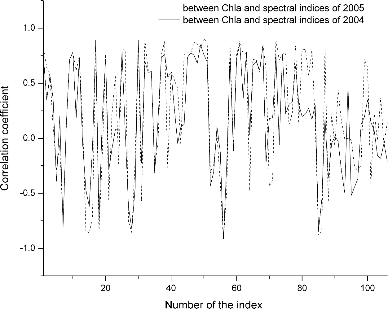 Correlation coefficients in 2004 were sorted from high to low and the top 10 are listed in Table 4, where . With regard to wavelengths, the sensitive reflectance to Chla mainly focused at 450, 550, 670 to 700, 800 nm or the nearby location. In terms of spectral indices, RARSa had the highest sensitivity to Chla. The top three highly correlated spectral indices were all composed by the band ratio of the reflectance peak near 700 nm and the reflectance trough near 670 nm, demonstrating the effectiveness of these two bands for Chla estimation in turbid water. Table 4Spectral indices highly correlated with lnChla in the dataset of 2004 (p<0.001).
The combinations of spectral indices, including band difference, band ratio and band normalization, were calculated based on the dataset of 2004. The top five highly correlated difference and ratio combinations are shown in Table 5, where . Results show that the difference and ratio of spectral indices generally had higher correlation with Chla than a single spectral index, and the performance of band ratio was slightly better than that of band difference. The ratio of the red/green pigment index31 and the ratio analysis of reflectance spectra56 (RGI/RARSa) has the highest correlation (0.94) with lnChla, better than RARSa (), as shown in Table 4. Table 5Difference and ratio combinations highly correlated with lnChla in the dataset of 2004.
The correlation coefficients between lnChla and the normalized combination of the spectral index pairs were calculated and the top three are listed in Table 6, denoted as NR1, NR2, and NR3. They were highly correlated with lnChla (, ). Table 6Three normalized combinations highly correlated with lnChla in the dataset of 2004.
3.3.Estimation of Chla Based on Spectral IndexBased on the same dataset used in Sec. 3.2, the three normalized combinations, NR1, NR2, and NR3 (Table 6), as well as the RARSa (Table 4) and RGI/ RARSa (Table 5) were used for model building. Results are shown in Table 7. Table 7Regression models between the spectral indices (NR1, NR2, NR3, RARSa, RGI/RARSa) and lnChla in the dataset of 2004 (p<0.0001).
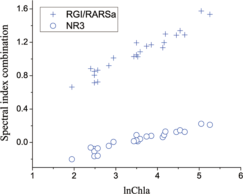
In the comparison between the value and RMSEs of NR1, NR2, and NR3, NR1 had the best fitting accuracy and NR3 had the lowest RMSE (Table 7). The fitting accuracy of NR1 was slightly better than NR3, but its RMSE and residual variation were larger. The residual diagnostics plots of NR1 and NR3 (Fig. 4) indicated that the residuals of NR1 showed heteroscedasticity as Chla changed, and more points in NR1 deviated from the straight line of its Q-Q plot [Fig. 4(a)]. Comparatively, NR3 fulfilled the requirement of regression analysis better than NR1 [Fig. 4(b)]. Fig. 4Residual diagnostics of the regression models of NR1 (a) and NR3 (b). The residual diagnostics include the homogeneity test of variance and the normality test of residuals. 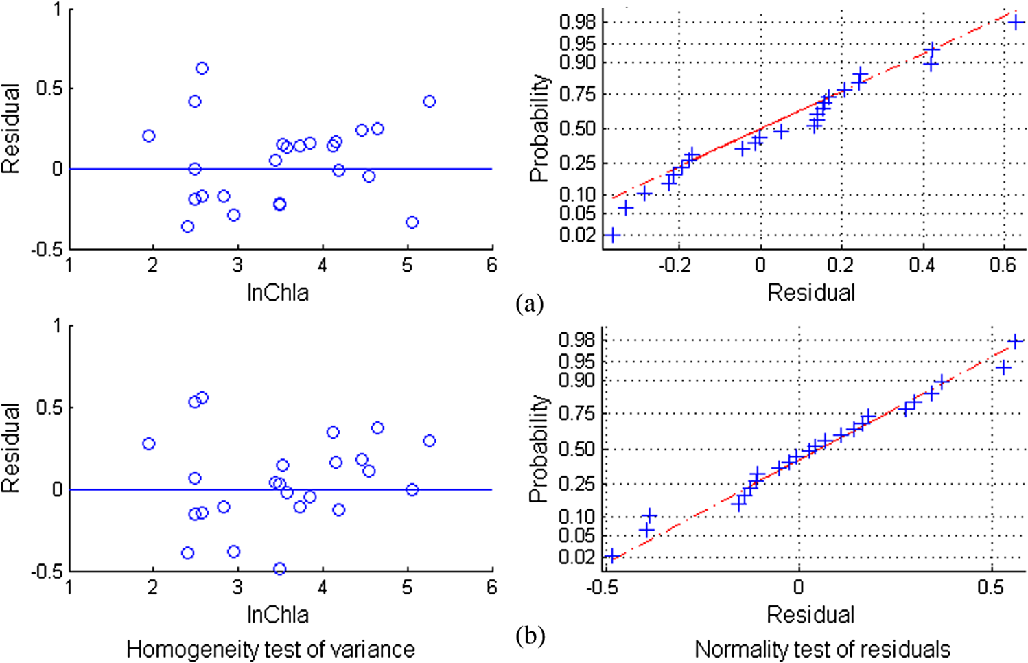 The results of RARSa and RGI/RARSa were then compared, and the results of the comparison are also shown in Table 7. Results showed that the RGI/RARSa had a higher fitting accuracy () than NR3 (). However, the scatter plot between RGI/RARSa and NR3 with lnChla (Fig. 5) showed that the variation of RGI/ RARSa was larger than NR3, indicating that the value of the RGI/RARSa ratio was higher and had a greater variation in sample distribution and that the NR3 value was lower and had a smaller variation. The NR3 was more stable with the change in lnChla. Therefore, NR3 was selected as the optimal index and called the normal chlorophyll index (NCI), . The Chla estimation model was , with ARE of 18.27%, and RMSE of . 3.4.Model ValidationDatasets of 2005, 2010, and 2011 were used for model validation. First, Chla was directly estimated using the model of , and their models were denoted as DV1, DV2, and DV3. Then, the model was reparameterized by rebuilding the regression models between the lnChla and NCI derived from the three datasets and then the Chla was estimated. The models were denoted as RV1, RV2, and RV3. Figure 6 shows the scatter plots between the estimated and measured Chla of the three datasets. Fig. 6Validation results of the NCI model by datasets of 2005 (a), 2010 (b), and 2011 (c). Validation process includes the direct Chla estimation from the 2004 model (DV1, DV2, and DV3), and the Chla estimation after reparameterization of the NCI model based on new datasets (RV1, RV2, and RV3).  By using the model of 2004 directly, the validation result by dataset of 2005 was satisfactory [DV1 in Fig. 6(a)], with RMSE of and ARE of 34.75%. This condition may be attributed to the consistency between these two datasets in July to August of 2004 and 2005. The standard deviations of the relative error in the NCI models for 2004 and 2005 were 0.216 and 0.242, respectively. However, although the distribution trend of the model was consistent with the measured Chla, Chla was generally underestimated when the model was directly validated using the datasets of 2010 and 2011 [DV2 in Fig. 6(b) and DV3 in Fig. 6(c)]. When the coefficients of the model were refitted using the calculated NCI and Chla in the new datasets, the estimated and measured Chla in the three datasets were consistent with each other (RV1, RV2, and RV3 in Fig. 6) and most samples were within the error line of . The RMSEs between the estimated Chla and the measured Chla for 2005, 2010, and 2011 were 10.39, 11.87, and , respectively. These results demonstrated the usability of NCI in the new datasets for the remote sensing mapping of Chla in a water body. 3.5.Model ApplicationTo verify the application of NCI index model in hyperspectral sensors, the Hyperion and CHRIS band reflectances were first simulated using the in situ spectra data in 2004 and 2005 according to the method mentioned in Sec. 2.5. Both Hyperion and CHRIS have four spectral channels consistent with the 550, 675, 690, and 700 nm of NCI, the basic parameters of which are shown in Table 8. The NCI was first calculated using the Hyperion band reflectance simulated by the in situ data in 2004 and 2005, whereas data in 2004 were used for model building and data in 2005 were used for model validation. Figure 7(a) shows the regression model between NCI and lnChla in 2004 and also the model accuracy, including , RMSE, and ARE. Figure 7(b) shows the validation results by directly using this model in 2005 data and also the validation accuracy of RMSE and ARE, calculated by the estimated results and the measured Chla. Similarly, Fig. 7(c) shows the NCI regression model using the CHRIS band reflectance simulated using the in situ data in 2004 and Fig. 7(d) shows the model validation result in 2005. Fig. 7The NCI model and validation results using simulated Hyperion/CHRIS data. Model result in 2004 (a) and validation result in 2005 (c) using simulated Hyperion data; Model result in 2004 (b) and validation result in 2005 (d) using simulated CHRIS data. 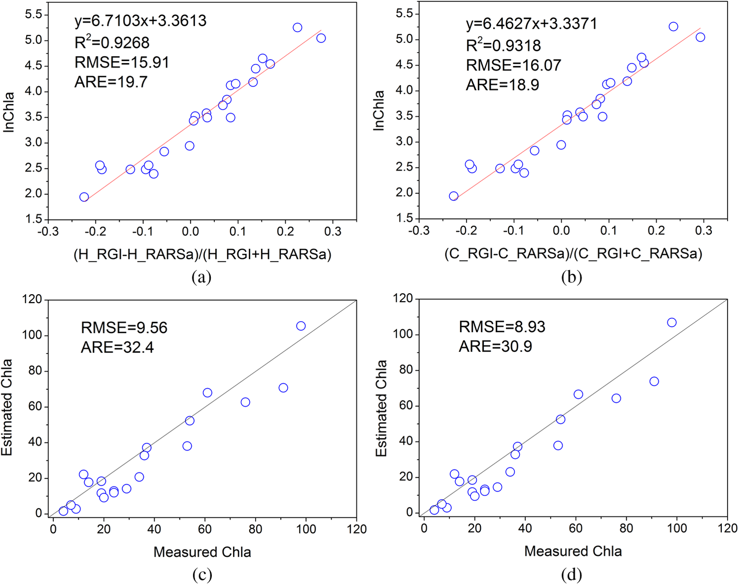 The accuracy of the NCI model using hyperspectral data is satisfactory, with and . The accuracy of the model built by the simulated hyperspectral data is better than that of using the in situ spectra (Table 7). Meanwhile, the estimation results are also satisfactorily in line with the measured Chla in 2005 using simulation data from both sensors [Figs. 7(c) and 7(d)], with . These results indicated that the NCI model can be used to estimate the Chla in Taihu lake using the Hyperion/EO-1 and CHRIS/PROBA spectra data with an accurate atmospheric correction of water body. This index will also have good usability in other hyperspectral satellite images with similar channel settings. 4.Discussion4.1.Model Performance of NCIWith regard to Taihu Lake, Le et al.12 stated that the optimal positions for the three-band model are 660, 692, and 740 nm, and the optimal positions for the four-band model are 662, 693, 740, and 705 nm. When the three- and four-band models were directly used without reparameterization of the new datasets in this study, the performance was poor (not shown). This result is similar to the results from previous studies.82,83 Based on the data obtained in July to August, 2004, the three- and four-band combinations were compared with NCI. The regression parameters between and were first refitted with Chla in 2004, and the optimal three- and four-band positions were then tuned to calibrate the model. Table 9 shows the results of the three- and four-band models after reparameterization and model calibration, and Fig. 8 shows their residual diagnostic plots. Table 8Hyperion’s and CHRIS’s band parameters near 550,675,690, and 700 nm.
Table 9Model and test results of the three- and four-band models after reparameterization and calibration in the dataset of 2004 (p<0.0001).
Fig. 8Test of variance homogeneity and residual normality of the three- and four-band algorithms after model reparameterization (a, c) and band tuning (b, d). 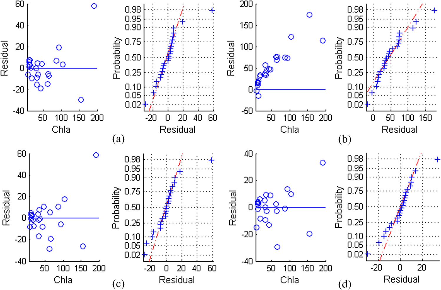 Table 9 shows that the models of the previous three- and four-band combinations after reparameterization (; ) were less significant than the NCI model (; ). Both the three- and four-band models achieved superior results after model calibration by band tuning, whereas the four-band model (; ) had a better estimation than NCI. However, the residual diagnostics plots (Fig. 8) showed that the residuals of the three- and four-band models were clearly non-normal and increased with Chla. The samples with lower and higher Chla had a larger deviation. Moreover, the error variance was correlated with Chla, indicating the residuals heteroscedasticity and the necessity for data transformation.77 Comparatively, the residual diagnostics of the NCI model [Fig. 4(b)] was better, indicating its robust performance in Chla prediction. The robustness of the NCI model can be explained from two aspects. The first is the logarithmic transformation of Chla before model building, which guarantees data normality. After data transformation, the model is better than directly using regression analysis. Previous studies83,84 demonstrated the same result. Regression models between the three- and four-band combinations and lnChla were also constructed to further verify the effect of data transformation. The reparameterized and calibrated three- and four-band models had poorer residual diagnostics results than the NCI, except for the calibrated three-band model (not shown). However, in this calibrated model , the third band found in the range of 450 to 800 nm did not confirm the assumption that it is the spectral region minimally affected by pigment absorption and can compensate for the variability in the backscattering between samples.9 If the searching ranges of , , and were reset into 658 to 676 nm, 691 to 735 nm, and 723 to 780 nm, respectively, according to Gitelson et al.,10,15 although the 664, 716, and 768 nm would be the last optimal bands, the residual diagnostic result of the calibrated model would still be poorer than that of NCI. The second aspect that can explain the robustness of the NCI model is the stable wavelengths used in this integrated index. Using the characteristic bands obtained from the vegetation index tested by Chappelle et al.56 and Zarco-Tejada et al.,31 the NCI proposed in this study was robust because it achieved satisfactory results when validated by multiple datasets. Comparatively, the three- or four-band combinations based on a small number of datasets did not perform well during validation, thus requiring band tuning in new datasets. Numerous results, including those of this study and Gitelson et al.,10,15 showed the necessity of model calibration of the three-band algorithm to make it suitable to new datasets. The three- and four-band models constructed by specific dataset may not fulfill the model assumptions when applied to other water bodies with different optical properties, thus producing unfavorable model diagnostics and inapplicable validation in new datasets. The estimation model based on NCI had a better residual diagnostics result, indicating that it is robust enough to be used in multiple datasets in Taihu Lake. 4.2.NCI and ChlaThe spectral reflectance of green plants is primarily affected by leaf color, cell structure, and plant moisture. The typical spectral curves of green plants are as follows: a small reflectance peak near 550 nm with reflectance of 10% to 20%; two obvious reflectance troughs near 450 and 670 nm owing to the strong absorption of pigment concentration; and a sharp increase of reflectance from 700 to 800 nm, leading to an obvious slope called “red edge.” Given a wide range of leaf greenness, the maximum sensitivity to Chla was found at 550 to 560 nm and 700 to 710 nm;85,86 its correlation with Chla at these two bands was larger than 675 nm, and the reciprocal reflectance near 550 and 700 nm was proportional to Chla.18,85 The reflectance at 670 nm decreased sharply when Chla increased up to 3 to . Thereafter, R670 was almost pigment-concentration independent. R670 can thus be used as a reference. However, the reflectance peak in the NIR area (larger than 750 nm) was insensitive to Chla.85 The ratio may amplify the differences between the spectra at specific bands due to absorption maxima and minima of the photosynthetic pigments.56 The band ratio of 675 and 700 nm (RARSa) was found to have a strong linear relationship with Chla () in the leaves of soybean.56 The red and green pigment index RGI () was used to estimate the pigment concentration of the leaf.31 The spectrum above water surface is affected by the absorption and scattering of water and particles in it, primarily including phytoplankton, suspended sediment, and CDOM. The four characteristic bands related to chlorophyll are the blue, green, red, and NIR bands in water color remote sensing.7,87–89 The ratio of the reflectance peak near 700 nm and the reflectance trough near 675 nm are proven to be most sensitive to Chla in turbid waters of different trophic states,6,17 which makes RARSa () reasonable. Moreover, the R690 in NCI can be regarded as the fluorescence peak because the fluorescence peak is around 690 nm, but can vary from 685 to 695 nm,90 or be constant at .91 Studies showed that normalizing the fluorescence peak near 700 nm to the reflectance value of the global maximum of the spectrum at green peak can accurately predict Chla,6,70 making RGI () reasonable. Although RARSa and RGI are proven to be theoretically effective in Chla estimation, the normalized combination of these two indices-NCI is optimal because of its robust performance as Chla changes (Fig. 5). The first advantage of NCI is the information supplementary of low Chla in the hyperspectral reflectance that cannot be fully expressed by the red-NIR spectrum by using the green band. Accurate estimates of low Chla using fluorescence algorithms, such as FLH and maximum chlorophyll index,92 or the red-NIR algorithms,17 are unavailable in oligotrophic and some mesotrophic lakes. Thus, the green band was additionally used because the blue and green bands in the OC2-OC4 algorithms were successfully applied to retrieve 0 to of Chla in optically complex waters. The second advantage of the NCI is that the feature wavelengths of 550, 675, 690, and 700 nm have all been set in hyperspectral sensors, such as EO-1/Hyperion, HJ1/HSI, PHILLS/HICO, and so on. Compared with the NCI, the commonly used three- or four- band models always require a reflectance longer than 750 nm. However, obtaining reliable estimates of reflectance at these wavelengths is a difficult task based on existing atmospheric correction schemes for turbid waters.16 Moreover, unlike previous studies on Chla estimation based on the spectra data obtained from July to August, 2004, in Taihu Lake, including the ratio,93 the three-band combination94or the band normalized combination,84 the NCI model proposed in this study was tested by regression diagnostics and validated by multiple datasets, thus guaranteeing more reliability. 5.ConclusionBased on the 106 spectral indices used in the vegetation remote sensing, this study first calculated the spectral indices based on the in situ spectra from July to August 2004, in Taihu Lake, China. The sensitivity of the spectral indices and their band combinations to the logarithmic transformation of Chla (lnChla) was then analyzed and compared. The integrated spectral index, NCI [], was found to be highly correlated with Chla, demonstrating its potential use in Chla estimation in turbid waters. Based on the NCI, a new Chla estimation model was constructed based on the 2004 data, which is , with of 0.92 and RMSE of . When the model was validated using the datasets of July to August 2005, September 2010, and September 2011, the model after reparameterization yielded low RMSEs between measured and estimated Chla, which were 10.39, 11.87, and , respectively. Compared with the three- and four-band models, the residuals’ diagnostics of the NCI model were significantly better, indicating the robustness of the model and its satisfactory validation performance in multiple datasets. Using the Hyperion/CHRIS band reflectance simulated by the in situ spectra data, model results in 2004 and validation results in 2005 were both satisfactory, showing good applicability of the NCI model. This study indicates that the abundant results from vegetation remote sensing have a great potential for Chla estimation in turbid waters. The NCI proposed in this study with stable band positions and robust model performance can be preferably used for Chla estimation in turbid waters. The Chla range suitable to NCI in this study is from 4 to . The usability of NCI out of this range will be discussed in future research. Given that the four datasets were all collected from Taihu Lake, one of the limitations of this study is that the calibration and validation datasets only contain a part of the optical properties of natural turbid waters. We suggest calibration and validation of the algorithms based on more field-measured data. AcknowledgmentsThe study was jointly supported by the National Natural Science Foundation of China grant (No. 40771152), the Natural Science Foundation of the Jiangsu Higher Education Institutions of China (09KJA420001). We would like to express our gratitude to Jiao Hongbo, Liu Ke, Gong Shaoqi, Xu Ning, Wang Lei, Zhang Xiaowei, Zhou Yu, and Sun Xiaopeng for their participation in the field and to Zhang Jing for her work in the laboratory. ReferencesS. Sathyendranath,
“Remote sensing of ocean colour in coastal, and other optically-complex, waters,”
MacNab Print, Dartmouth, Canada
(2000). Google Scholar
A. G. DekkerR. J. VosS. W. M. Peters,
“Analytical algorithms for lake water TSM estimation for retrospective analyses of TM and SPOT sensor data,”
Int. J. Remote Sens., 23
(1), 15
–35
(2002). http://dx.doi.org/10.1080/01431160010006917 IJSEDK 0143-1161 Google Scholar
D. G. George,
“The airborne remote sensing of phytoplankton chlorophyll in the lakes and tarns of the English Lake District,”
Int. J. Remote Sens., 18
(9), 1961
–1975
(1997). http://dx.doi.org/10.1080/014311697217972 IJSEDK 0143-1161 Google Scholar
J. E. O’Reillyet al.,
“Ocean color chlorophyll algorithms for SeaWiFS,”
J. Geophys. Res., 103
(C11), 24937
–24953
(1998). http://dx.doi.org/10.1029/98JC02160 JGREA2 0148-0227 Google Scholar
A. MorelL. Prieur,
“Analysis of variations in ocean color,”
Limnol. Oceanogr., 22
(4), 709
–722
(1977). http://dx.doi.org/10.4319/lo.1977.22.4.0709 LIOCAH 0024-3590 Google Scholar
A. A. Gitelson,
“The peak near 700 nm on radiance spectra of algae and water: relationships of its magnitude and position with chlorophyll concentration,”
Int. J. Remote Sens., 13
(17), 3367
–3373
(1992). http://dx.doi.org/10.1080/01431169208904125 IJSEDK 0143-1161 Google Scholar
L. H. HanD. C. Rundquist,
“Comparison of NIR/RED ratio and first derivative of reflectance in estimating algal-chlorophyll concentration: a case study in a turbid reservoir,”
Remote Sens. Environ., 62
(3), 253
–261
(1997). http://dx.doi.org/10.1016/S0034-4257(97)00106-5 RSEEA7 0034-4257 Google Scholar
J. F. R. GowerR. DoerfferG. A. Borstad,
“Interpretation of the 685 nm peak in water-leaving radiance spectra in terms of fluorescence, absorption and scattering, and its observation by MERIS,”
Int. J. Remote Sens., 20
(9), 1771
–1786
(1999). http://dx.doi.org/10.1080/014311699212470 IJSEDK 0143-1161 Google Scholar
G. Dall’OlmoA. A. GitelsonD. C. Rundquist,
“Towards a unified approach for remote estimation of chlorophyll-a in both terrestrial vegetation and turbid productive waters,”
Geophys. Res. Lett., 30
(18), 1938
(2003). http://dx.doi.org/10.1029/2003GL018065 GPRLAJ 0094-8276 Google Scholar
A. A. GitelsonJ. F. SchallesC. M. Hladik,
“Remote chlorophyll-a retrieval in turbid, productive estuaries: Chesapeake Bay case study,”
Remote Sens. Environ., 109
(4), 464
–472
(2007). http://dx.doi.org/10.1016/j.rse.2007.01.016 RSEEA7 0034-4257 Google Scholar
Y. C. WeiG. X. WangJ. Z. Huang,
“Validation of the three-band chlorophyll-a inversion model in turbid water: the case of Taihu Lake, China,”
Proc. SPIE, 7678 767809
(2010). http://dx.doi.org/10.1117/12.849818 PSISDG 0277-786X Google Scholar
C. F. Leet al.,
“A four-band semi-analytical model for estimating chlorophyll a in highly turbid lakes: The case of Taihu Lake, China,”
Remote Sens. Environ., 113
(6), 1175
–1182
(2009). http://dx.doi.org/10.1016/j.rse.2009.02.005 RSEEA7 0034-4257 Google Scholar
C. P. Kuchinkeet al.,
“Spectral optimization for constituent retrieval in Case 2 waters II: Validation study in the Chesapeake Bay,”
Remote Sens. Environ., 113
(6), 610
–621
(2009). http://dx.doi.org/10.1016/j.rse.2008.11.002 RSEEA7 0034-4257 Google Scholar
A. Magnusonet al.,
“Bio-optical model for Chesapeake Bay and the middle Atlantic bight,”
Estuarine Coastal Shelf Sci., 61
(3), 403
–424
(2004). http://dx.doi.org/10.1016/j.ecss.2004.06.020 ECSSD3 0272-7714 Google Scholar
A. A. Gitelsonet al.,
“A simple semi-analytical model for remote estimation of chlorophyll-a in turbid waters: validation,”
Remote Sens. Environ., 112
(9), 3582
–3593
(2008). http://dx.doi.org/10.1016/j.rse.2008.04.015 RSEEA7 0034-4257 Google Scholar
W. J. Moseset al.,
“Estimation of chlorophyll-a concentration in case II waters using MODIS and MERIS data-successes and challenges,”
Environ. Res. Lett., 4
(4), 045005
(2009). http://dx.doi.org/10.1088/1748-9326/4/4/045005 ERLNAL 1748-9326 Google Scholar
D. Odermattet al.,
“Review of constituent retrieval in optically deep and complex waters from satellite imagery,”
Remote Sens. Environ., 118 116
–126
(2012). http://dx.doi.org/10.1016/j.rse.2011.11.013 RSEEA7 0034-4257 Google Scholar
A. A. GitelsonY. GritzM. N. Merzlyak,
“Relationships between leaf chlorophyll content and spectral reflectance and algorithms for non-destructive chlorophyll assessment in higher plant leaves,”
J. Plant Physiol., 160
(3), 271
–282
(2003). http://dx.doi.org/10.1078/0176-1617-00887 JPPHEY 0176-1617 Google Scholar
B. J. YoderR. E. Pettigrew-Crosby,
“Predicting nitrogen and chlorophyll content and concentrations from reflectance spectra (400–2500 nm) at leaf and canopy scales,”
Remote Sens. Environ., 53
(3), 199
–211
(1995). http://dx.doi.org/10.1016/0034-4257(95)00135-N RSEEA7 0034-4257 Google Scholar
J. E. McMurtey IIIet al.,
“Distinguish nitrogen fertilization levels in field corns (Zea mays L.) with actively induced fluorescence and passive reflectance measurements,”
Remote Sens. Environ., 47
(1), 36
–44
(1994). http://dx.doi.org/10.1016/0034-4257(94)90125-2 RSEEA7 0034-4257 Google Scholar
R. L. PearsonL. D. Miller,
“Remote mapping of standing crop biomass for estimation of the productivity of the shortgrass prairie, Pawnee National Grasslands, Colorado,”
in Proc. 8th International Symp. Remote Sensing of the Environment,
1355
–1379
(1972). Google Scholar
A. A. GitelsonM. N. Merzylac,
“Spectral reflectance changes associate with autumn senescence of Aesculus hippocastanum L. and Acer platanoides L. leaves,”
J. Plant Physiol., 143
(3), 286
–292
(1994). http://dx.doi.org/10.1016/S0176-1617(11)81633-0 JPPHEY 0176-1617 Google Scholar
S. MishraD. R. Mishra,
“Normalized difference chlorophyll index: a novel model for remote estimation of chlorophyll–a concentration in turbid productive waters,”
Remote Sens. Environ., 117 394
–406
(2012). http://dx.doi.org/10.1016/j.rse.2011.10.016 RSEEA7 0034-4257 Google Scholar
J. W. Rouseet al.,
“Monitoring vegetation systems in the Great Plains with ERTS,”
in Third ERTS Symp.,
309
–317
(1973). Google Scholar
B. Q. QinW. P. HuW. M. Chen, Water Environment Evolution Process and Mechanism of Taihu Lake, Science Press, Beijing
(2004). Google Scholar
J. L. MuellerG. S. FargionC. R. McClain,
“Radiometric measurements and data analysis protocols,”
NASA/TM-2003-Ocean Optics Protocols for Satellite Ocean Color Sensor Validation, Goddard Space Flight Center (2003). Google Scholar
Y. C. WeiG. X. WangC. M. Cheng,
“Noise removal in spectrum above water surface using kernel regression smoothing,”
J. Nanjing Normal Univ., 33
(3), 97
–102
(2010). http://dx.doi.org/10.3969/j.issn.1001-4616.2010.03.019 NSXZEN 1001-4616 Google Scholar
A. Viñaet al.,
“Comparison of different vegetation indices for the remote assessment of green leaf area index of crops,”
Remote Sens. Environ., 115
(12), 3468
–3478
(2011). http://dx.doi.org/10.1016/j.rse.2011.08.010 RSEEA7 0034-4257 Google Scholar
F. BaretG. Guyot,
“Potentials and limits of vegetation indices for LAI and APAR assessment,”
Remote Sens. Environ., 35
(2), 161
–173
(1991). http://dx.doi.org/10.1016/0034-4257(91)90009-U RSEEA7 0034-4257 Google Scholar
P. J. Zarco-Tejadaet al.,
“Scaling-up and model inversion methods with narrow-band optical indices for chlorophyll content estimation in closed forest canopies with hyperspectral data,”
IEEE Trans. Geosci. Remote Sens., 39
(7), 1491
–1507
(2001). http://dx.doi.org/10.1109/36.934080 IGRSD2 0196-2892 Google Scholar
P. J. Zarco-Tejadaet al.,
“Assessing vineyard condition with hyperspectral indices: Leaf and canopy reflectance simulation in a row-structured discontinuous canopy,”
Remote Sens. Environ., 99
(3), 271
–287
(2005). http://dx.doi.org/10.1016/j.rse.2005.09.002 RSEEA7 0034-4257 Google Scholar
C. BuschmanE. Nagel,
“In vivo spectroscopy and internal optics of leaves as a basis for remote sensing of vegetation,”
Int. J. Remote Sens., 14
(4), 711
–722
(1993). http://dx.doi.org/10.1080/01431169308904370 IJSEDK 0143-1161 Google Scholar
M. S. Kimet al.,
“The use of high spectral resolution bands for estimating absorbed photosynthetically active radiation (A par),”
in Phys. Meas. Signatures Remote Sens.,
299
–306
(1994). Google Scholar
P. J. Zarco-Tejadaet al.,
“Chlorophyll fluorescence effects on vegetation apparent reflectance: I. Leaf-level measurements and simulation of reflectance and transmittance spectra,”
Remote Sens. Environ., 74
(3), 582
–595
(2000). http://dx.doi.org/10.1016/S0034-4257(00)00148-6 RSEEA7 0034-4257 Google Scholar
G. A. Carter,
“Ratios of leaf reflectance in narrow wavebands as indicators of plant stress,”
Int. J. Remote Sens., 15
(3), 697
–704
(1994). http://dx.doi.org/10.1080/01431169408954109 IJSEDK 0143-1161 Google Scholar
G. A. CarterT. R. DellW. G. Cibula,
“Spectral reflectance characteristics and digital imagery of a pine needle blight in the southeastern United States,”
Can. J. For. Res., 26
(3), 402
–407
(1996). http://dx.doi.org/10.1139/x26-045 CJRSDP 0703-8992 Google Scholar
G. L. MaireC. FrancoisE. Dufrene,
“Towards universal broad leaf chlorophyll indices using PROSPECT simulated database and hyperspectral reflectance measurements,”
Remote Sens. Environ., 89
(1), 1
–28
(2004). http://dx.doi.org/10.1016/j.rse.2003.09.004 RSEEA7 0034-4257 Google Scholar
C. F. Jordan,
“Derivation of leaf area index from quality of light on the forest floor,”
Ecology, 50
(4), 663
–666
(1969). http://dx.doi.org/10.2307/1936256 ECOLAR 0012-9658 Google Scholar
B. Datt,
“Remote sensing of chlorophyll a, chlorophyll b, chlorophyll and total carotenoid content in eucalyptus leaves,”
Remote Sens. Environ., 66
(2), 111
–121
(1998). http://dx.doi.org/10.1016/S0034-4257(98)00046-7 RSEEA7 0034-4257 Google Scholar
C. S. T. Daughtryet al.,
“Estimating corn leaf chlorophyll concentration from leaf and canopy reflectance,”
Remote Sens. Environ., 74
(2), 229
–239
(2000). http://dx.doi.org/10.1016/S0034-4257(00)00113-9 RSEEA7 0034-4257 Google Scholar
A. A. GitelsonY. J. KaufmanM. N. Merzlyak,
“Use of a green channel in remote sensing of global vegetation from EOS-MODIS,”
Remote Sens. Environ., 58
(3), 289
–298
(1996). http://dx.doi.org/10.1016/S0034-4257(96)00072-7 RSEEA7 0034-4257 Google Scholar
B. Datt,
“A new reflectance index for remote sensing of chlorophyll content in higher plants: tests using Eucalyptus leaves,”
J. Plant Physiol., 154
(1), 30
–36
(1999). http://dx.doi.org/10.1016/S0176-1617(99)80314-9 JPPHEY 0176-1617 Google Scholar
H. K. Lichtenthaleret al.,
“Detection of vegetation stress via a new high resolution fluorescence imaging system,”
J. Plant Physiol., 148
(5), 599
–612
(1996). http://dx.doi.org/10.1016/S0176-1617(96)80081-2 JPPHEY 0176-1617 Google Scholar
A. MaccioniG. AgatiP. Mazzinghi,
“New vegetation indices for remote measurement of chlorophylls based on leaf directional reflectance spectra,”
J. Photochem. Photobiol. B, 61
(1), 52
–61
(2001). http://dx.doi.org/10.1016/S1011-1344(01)00145-2 JPPBEG 1011-1344 Google Scholar
D. Haboudaneet al.,
“Hyperspectral vegetation indices and novel algorithms for predicting green LAI of crop canopies: modeling and validation in the context of precision agriculture,”
Remote Sens. Environ., 90
(3), 337
–352
(2004). http://dx.doi.org/10.1016/j.rse.2003.12.013 RSEEA7 0034-4257 Google Scholar
D. A. SimsJ. A. Gamon,
“Relationships between leaf pigment content and spectral reflectance across a wide range of species, leaf structures and developmental stages,”
Remote Sens. Environ., 81
(2), 337
–354
(2002). http://dx.doi.org/10.1016/S0034-4257(02)00010-X RSEEA7 0034-4257 Google Scholar
J. Qiet al.,
“A modified soil adjusted vegetation index,”
Remote Sens. Environ., 48
(2), 119
–126
(1994). http://dx.doi.org/10.1016/0034-4257(94)90134-1 RSEEA7 0034-4257 Google Scholar
J. M. Chen,
“Evaluation of vegetation indices and modified simple ratio for boreal applications,”
Can. J. Remote Sens., 22
(3), 229
–242
(1996). CJRSDP 0703-8992 Google Scholar
J. PeňuelasJ. A. GamonA. L. Fredeen,
“Reflectance indices associated with physiological changes in nitrogen and water limited sunflower leaves,”
Remote Sens. Environ., 48
(2), 135
–146
(1994). http://dx.doi.org/10.1016/0034-4257(94)90136-8 RSEEA7 0034-4257 Google Scholar
J. D. Barneset al.,
“A reappraisal of the use of DMSO for the extraction and determination of chlorophylls a and b in lichens and higher plants,”
Environ. Exp. Botany, 32
(2), 85
–100
(1992). http://dx.doi.org/10.1016/0098-8472(92)90034-Y EEBODM 0098-8472 Google Scholar
G. RondeauxM. StevenF. Baret,
“Optimization of soil adjusted vegetation indices,”
Remote Sens. Environ., 55
(2), 95
–107
(1996). http://dx.doi.org/10.1016/0034-4257(95)00186-7 RSEEA7 0034-4257 Google Scholar
N. R. Raoet al.,
“Estimation of leaf total chlorophyll and nitrogen concentrations using hyperspectral satellite imagery,”
J. Agri. Sci., 146
(1), 65
–75
(2008). http://dx.doi.org/http://dx.doi.org/10.1017/S0021859607007514 Google Scholar
G. A. Blackburn,
“Quantifying chlorophylls and carotenoids at leaf and canopy scales; an evaluation of some hyperspectral approaches,”
Remote Sens. Environ., 66
(3), 273
–285
(1998). http://dx.doi.org/10.1016/S0034-4257(98)00059-5 RSEEA7 0034-4257 Google Scholar
J. A. GamonJ. PenuelasC. B. Field,
“A narrow-waveband spectral index that tracks diurnal changes in photosynthetic efficiency,”
Remote Sens. Environ., 41
(1), 35
–44
(1992). http://dx.doi.org/10.1016/0034-4257(92)90059-S RSEEA7 0034-4257 Google Scholar
A. A. GitelsonC. BuschmannH. K. Lichtenthaler,
“The chlorophyll fluorescence ratio F735/F700 as an accurate measure of the chlorophyll content in plants,”
Remote Sens. Environ., 69
(3), 296
–302
(1999). http://dx.doi.org/10.1016/S0034-4257(99)00023-1 RSEEA7 0034-4257 Google Scholar
E. W. ChappelleM. S. KimJ. E. McMurtrey III,
“Ratio analysis of reflectance spectra (RARS): an algorithm for the remote estimation of the concentrations of chlorophyll a, chlorophyll b and carotenoids in soybean leaves,”
Remote Sens. Environ., 39
(3), 239
–247
(1992). http://dx.doi.org/10.1016/0034-4257(92)90089-3 RSEEA7 0034-4257 Google Scholar
R. N. Merton,
“Monitoring community hysteresis using spectral shift analysis and the red-edge vegetation stress index,”
in Proc. Seventh Annual JPL Airborne Earth Science Workshop,
(1998). Google Scholar
A. R. Huete,
“A soil-adjusted vegetation index (SAVI),”
Remote Sens. Environ., 25
(3), 295
–309
(1988). http://dx.doi.org/10.1016/0034-4257(88)90106-X RSEEA7 0034-4257 Google Scholar
J. Peňuelaset al.,
“Reflectance assessment of mite effects on apple trees,”
Int. J. Remote Sens., 16
(14), 2727
–2733
(1995). http://dx.doi.org/10.1080/01431169508954588 IJSEDK 0143-1161 Google Scholar
C. D. ElvidgeC. Zhikang,
“Comparison of broad-band and narrow-band red and near-infrared vegetation indices,”
Remote Sens. Environ., 54
(1), 38
–48
(1995). http://dx.doi.org/10.1016/0034-4257(95)00132-K RSEEA7 0034-4257 Google Scholar
I. FilellaJ. Penuelas,
“Red edge position and shapes as indicators of plant chlorophyll content, biomass and hydric status,”
Int. J. Remote Sens., 15
(7), 1459
–1470
(1994). http://dx.doi.org/10.1080/01431169408954177 IJSEDK 0143-1161 Google Scholar
N. H. BrogeE. Leblanc,
“Comparing prediction power and stability of broadband and hyperspectral vegetation indices for estimation of green leaf area index and canopy chlorophyll density,”
Remote Sens. Environ., 76
(2), 156
–172
(2001). http://dx.doi.org/10.1016/S0034-4257(00)00197-8 RSEEA7 0034-4257 Google Scholar
D. Haboudaneet al.,
“Integrated narrow-band vegetation indices for prediction of crop chlorophyll content for application to precision agriculture,”
Remote Sens. Environ., 81
(2), 416
–426
(2002). http://dx.doi.org/10.1016/S0034-4257(02)00018-4 RSEEA7 0034-4257 Google Scholar
J. E. VogelmannB. N. RockD. M. Moss,
“Red edge spectral measurements from sugar maple leaves,”
Int. J. Remote Sens., 14
(8), 1563
–1575
(1993). http://dx.doi.org/10.1080/01431169308953986 IJSEDK 0143-1161 Google Scholar
A. A. GitelsonG. P. KeydanM. N. Merzlyak,
“Three-band model for noninvasive estimation of chlorophyll, carotenoids, and anthocyanin contents in higher plant leaves,”
Geophys. Res. Lett., 33
(11), 1
–5
(2006). http://dx.doi.org/10.1029/2006GL026457 GPRLAJ 0094-8276 Google Scholar
A. Hueteet al.,
“Overview of the radiometric and biophysical performance of the MODIS vegetation indices,”
Remote Sens. Environ., 83
(1), 195
–213
(2002). http://dx.doi.org/10.1016/S0034-4257(02)00096-2 RSEEA7 0034-4257 Google Scholar
J. L. RoujeanF. M. Breon,
“Estimating PAR absorbed by vegetation from bidirectional reflectance measurements,”
Remote Sens. Environ., 51
(3), 375
–384
(1995). http://dx.doi.org/10.1016/0034-4257(94)00114-3 RSEEA7 0034-4257 Google Scholar
A. A. Gitelsonet al.,
“Assessing carotenoid content in plant leaves with reflectance spectroscopy,”
Photochem. Photobiol., 75
(3), 272
–281
(2002). http://dx.doi.org/10.1562/0031-8655(2002)075<0272:ACCIPL>2.0.CO;2 PHCBAP 0031-8655 Google Scholar
A. A. Gitelson,
“Wide dynamic range vegetation index for remote quantification of biophysical characteristics of vegetation,”
J. Plant Physiol., 161
(2), 165
–173
(2004). http://dx.doi.org/10.1078/0176-1617-01176 JPPHEY 0176-1617 Google Scholar
D. Z. Zhaoet al.,
“The optimized spectral bands ratio for the relation of sun-induced chlorophyll fluorescence height with high chlorophyll a concentration of algal bloom waters,”
Acta Oceanologica Sinica, 27
(6), 146
–153
(2005). http://dx.doi.org/10.3321/j.issn:0253-4193.2005.06.019 AOSIEE 0253-505X Google Scholar
W. L. VosM. DonzeH. Bueteveld,
“On the reflectance spectrum of algae in water: the nature of the peak at 700 nm and its shift with varying concentration,”
Communications on Sanitary Engineering and Water Management, Delft, The Netherlands
(1986). Google Scholar
J. R. MillerE. W. Hare,
“Quantitative characterization of the vegetation red edge reflectance. 1. An inverted Gaussian reflectance model,”
Int. J. Remote Sens., 11
(10), 1775
–1795
(1990). http://dx.doi.org/10.1080/01431169008955128 IJSEDK 0143-1161 Google Scholar
S. ThiemannM. BergerH. Kaufmann,
“Feasibility study for lake water quality assessment using MIDORI AVNIR data,”
936
–938 IEEE International, Seattle, Washington
(1998). Google Scholar
P. GongR. L. PuR. C. Heald,
“Analysis of in situ hyperspectral data for nutrient estimation of giant sequoia,”
Int. J. Remote Sens., 23
(9), 1827
–1850
(2002). http://dx.doi.org/10.1080/01431160110075622 IJSEDK 0143-1161 Google Scholar
P. V. ZimbaA. A. Gitelson,
“Remote estimation of chlorophyll concentration in hyper-eutrophic aquatic systems: Model tuning and accuracy optimization,”
Aquaculture, 256
(1), 272
–286
(2006). http://dx.doi.org/10.1016/j.aquaculture.2006.02.038 AQCLAL 0044-8486 Google Scholar
R. H. Myers, Classical and Modern Regression with Applications, 2nd ed.Duxbury Press, Belmont, California
(1990). Google Scholar
X. Z. Wu, Modern Regression Model Diagnostic, China Statistics Press, Beijing
(2004). Google Scholar
E. J. MiltonK.Y. Choi,
“Estimating the spectral response function of the casi-2,”
in Annual Conference of the Remote Sensing and Photogrammetry Society, Remote Sensing and Photogrammetry Society,
1
–11
(2004). Google Scholar
C. Mike, CHRIS Data Format, Surrey Satellite Technology Limited, UK
(2008). Google Scholar
S. G. H. SimisS. W. M. PetersH. J. Gons,
“Remote sensing of the cyanobacterial pigment phycocyanin in turbid inland water,”
Limnol. Oceanogr., 50
(1), 237
–245
(2005). http://dx.doi.org/10.4319/lo.2005.50.1.0237 LIOCAH 0024-3590 Google Scholar
R. L. PuP. Gong, Hyperspectral Remote Sensing and its Applications, Higher Education, Beijing
(2000). Google Scholar
G. Dall’OlmoA. A. Gitelson,
“Effect of bio-optical parameter variability and uncertainties in reflectance measurements on the remote estimation of chlorophyll a concentration in turbid productive waters: Modeling results,”
Appl. Opt., 45
(15), 3577
–3592
(2006). http://dx.doi.org/10.1364/AO.45.003577 APOPAI 0003-6935 Google Scholar
Y. C. WeiG. X. WangH. Y. Sun,
“A logical problem in the building linear regression model on estimating chlorophyll-a concentration in lake based on the measured spectrum data,”
Math. Pract. Theory, 40
(18), 100
–110
(2010). 1000-0984 Google Scholar
Y. C. Weiet al.,
“The hyperspectral data monitoring model of chlorophyll-a of summer in Taihu Lake, China,”
J. Remote Sens., 11
(5), 756
–762
(2007). http://dx.doi.org/10.11834/jrs.200705103 Google Scholar
A. A. GitelsonM. N. Merzlyak,
“Signature analysis of leaf reflectance spectra: algorithm development for remote sensing of chlorophyll,”
J. Plant Physiol., 148
(3), 494
–500
(1996). http://dx.doi.org/10.1016/S0176-1617(96)80284-7 JPPHEY 0176-1617 Google Scholar
J. R. ThomasH. W. Gaussman,
“Leaf reflectance vs. leaf chlorophyll and carotenoid concentration for eight crops,”
Agron. J., 69
(5), 799
–802
(1977). http://dx.doi.org/10.2134/agronj1977.00021962006900050017x AGJOAT 0002-1962 Google Scholar
A. G. DekkerT. J. MalthusE. Seyhan,
“Quantitative modeling of inland water quality for high resolution MSS systems,”
IEEE Trans. Geosci. Remote Sens., 29
(1), 89
–95
(1991). http://dx.doi.org/10.1109/36.103296 IGRSD2 0196-2892 Google Scholar
L. H. Hanet al.,
“The spectral responses of algal chlorophyll in water with varying levels of suspended sediment,”
Int. J. Remote Sens., 15
(18), 3707
–3718
(1994). http://dx.doi.org/10.1080/01431169408954353 IJSEDK 0143-1161 Google Scholar
K. H. Mittenzweyet al.,
“Determination of chlorophyll a of inland waters on the basis of spectral reflectance,”
Limnol. Oceanogr., 37
(1), 147
–149
(1992). http://dx.doi.org/10.4319/lo.1992.37.1.0147 LIOCAH 0024-3590 Google Scholar
A. A. GitelsonY. Z. Yacobi,
“Reflectance in the red and near infra-red ranges of the spectrum as tool for remote chlorophyll estimation in inland waters-Lake Kinneret case study,”
in Electrical and Electronics Engineers in Eighteenth Convention of IEEE,
5.2.6/1
–5.2.6/5
(1995). Google Scholar
J. F. Schalles,
“Optical remote sensing techniques to estimate phytoplankton chlorophyll a concentrations in coastal waters with varying suspended matter and CDOM concentrations,”
Remote Sensing of Aquatic Coastal Ecosystem Processes, 27
–79 Springer, Netherlands
(2006). Google Scholar
L. Guanteret al.,
“Atmospheric correction of ENVISAT/MERIS data over inland waters: validation for European lakes,”
Remote Sens. Environ., 114
(3), 467
–480
(2010). http://dx.doi.org/10.1016/j.rse.2009.10.004 RSEEA7 0034-4257 Google Scholar
X. Z. ShuQ. YinD. B. Kuang,
“Relationship between algal chlorophyll concentration and spectral reflectance of inland water,”
J. Remote Sens., 4
(1), 41
–45
(2000). http://dx.doi.org/10.11834/jrs.20000108 Google Scholar
Y. Yanget al.,
“Retrieval of chlorophyll-a concentration in the turbid and eutrophic Taihu Lake,”
Geoinf. Sci., 11
(5), 597
–603
(2009). http://dx.doi.org/10.3724/SP.J.1047.2009.00597 1560-8999 Google Scholar
Biography Chunmei Cheng is a PhD candidate at the Key Lab of Virtual Geographic Environment, Ministry of Education in Nanjing Normal University of China. Her major is geographic information system, and her research interest is water color remote sensing.  Yuchun Wei is a professor at the Key Lab of Virtual Geographic Environment, Ministry of Education in Nanjing Normal University of China. He received his PhD degree at Nanjing Normal University in 2001. His research focuses on environmental remote sensing and image processing. |
|||||||||||||||||||||||||||||||||||||||||||||||||||||||||||||||||||||||||||||||||||||||||||||||||||||||||||||||||||||||||||||||||||||||||||||||||||||||||||||||||||||||||||||||||||||||||||||||||||||||||||||||||||||||||||||||||||||||||||||||||||||||||||||||||||||||||||||||||||||||||||||||||||||||||||||||||||||||||||||||||||||||||||||||||||||||||||||||||||||||||||||||||||||||||||||||||||||||||||||||||||||||||||||||||||||||||||||||||||||||||||||||||||||||||||||||||||||||||||||||||||||||||||||||||||||||||||||||||||||||||||||||||||||||||||||||||||||||||||