Soil moisture assessments for brown locust Locustana pardalina breeding potential using synthetic aperture radar

William T. Crooks; Robert A. Cheke

doi:10.1117/1.JRS.8.084898

18 March 2014 Soil moisture assessments for brown locust Locustana pardalina breeding potential using synthetic aperture radar

William T. Crooks, Robert A. Cheke

Author Affiliations +

Journal of Applied Remote Sensing, Vol. 8, Issue 1, 084898 (March 2014). https://doi.org/10.1117/1.JRS.8.084898

Abstract

Synthetic aperture radar (SAR) imagery was collected over a brown locust Locustana pardalina outbreak area to estimate soil moisture relevant to egg development. ERS-2/RadarSat overpasses and field studies enabled parameterization of surface roughness, volumetric soil moisture, soil texture, and vegetation cover. Data were analyzed both when the target area was assessed as nonvegetated and when treated as vegetated. For the former, using the integral equation model (IEM) and soil surface data combined with the sensitivity of the IEM to changes in surface roughness introduced an error of ∼±0.06 cm ³ cm ⁻³ in volumetric soil moisture. Comparison of the IEM modeling results with backscatter responses from the ERS-2/RadarSat imagery revealed errors as high as ±0.14 cm ³ cm ⁻³ , mostly due to IEM calibration problems and the impact of vegetation. Two modified versions of the water cloud model (WCM) were parameterized, one based on measurements of vegetation moisture and the other on vegetation biomass. A sensitivity analysis of the resulting model revealed a positive relationship between increases in both vegetation biomass and vegetation moisture and the backscatter responses from the ERS-2 and RadarSat sensors. The WCM was able to explain up to 80% of the variability found when the IEM was used alone.

1. Introduction

Locusts and grasshoppers (Orthoptera: Acrididae) are infamous pests responsible for destroying crops and pastures.¹^–³ All locust species require moist soil for oviposition and varying degrees of moisture at different times to allow their eggs to develop and hatch. For instance, desert locusts Schistocerca gregaria need at least 25 mm of rain to have fallen after their eggs have been laid to allow successful breeding,⁴ whereas other species, such as the Senegalese grasshopper Oedaleus senegalensis, can enter quiescence or diapause and their eggs may hatch as long as five years after being laid.⁵^,⁶ This is also true of the brown locust Locustana pardalina that occurs in southern Africa. Although remote sensing has been used both for research and operationally to detect green vegetation, for instance, as a proxy for the likelihood of desert locust presence,⁷^–¹⁰ an earlier warning system capable of detecting conditions suitable for the laying and hatching of eggs would be advantageous. Here we present results of a study addressing this issue using synthetic aperture radar (SAR) images of soil in habitats where the brown locust breeds in the Republic of South Africa.

Brown locusts persist as scattered populations in a semiarid outbreak area of $250,000 {km}^{2}$ in the Karoo regions of South Africa and southern Namibia,¹¹ whence they may spread into an invasion area of nearly 7 million ${km}^{2}$ across eight neighboring countries, as far north as the Zambezi River.¹² Kieser et al.¹³ described how land use practices and changing rainfall patterns in South Africa have led to the outbreak area being modified to extend further west and south-west than the zone described by Lea.¹⁴ Currently, there is no active field monitoring program to locate hopper bands, and control efforts, using broad-spectrum insecticides on congregated immature locusts or roosting mature swarms, rely on the legal requirement of farmers to report outbreaks on their property.¹⁵

The main hatching period of the brown locust in the Karoo begins with spring rains in September and continues into October. Fledging begins in December, and a second generation of eggs can be laid in January and a third in April.¹⁶ Egg pods with 10 to 82 eggs³ are laid and the incubation period can be as short as 10 to 20 days,¹⁷ depending on soil moisture availability and temperature. Temperatures need to exceed 8.5°C for eggs to develop, with an optimum temperature of $\sim 35 ° C$ .¹⁷ The role of moisture in egg development is considerably more complicated. Work by Matthée¹⁷ on the moisture dynamics of brown locust egg development highlighted several key factors, which are summarized below.

• For approximately the first nine days after oviposition, the eggs will develop with or without available moisture. Afterwards, if moisture is not available, the eggs become quiescent when they are drought tolerant since they can reduce their rate of moisture loss through evaporation. Provided that the egg moisture content does not fall below $\sim 40 %$ , the quiescent state can be broken by the presence of moisture, which the eggs then absorb. If this moisture is insufficient to stimulate hatching and these same eggs are again subjected to desiccation, they can then reenter a quiescent state.
• A proportion of eggs, dependent to some extent on the phase of the parent female as solitarious females lay mostly diapausing eggs—while gregarious females tend to lay nondiapausing eggs³—will enter diapause with the ability to remain dormant for an indefinite period provided that the eggs’ moisture content does not fall below $\sim 40 %$ . In this state, the eggs can absorb available moisture but will not proceed to full development even while nondiapause eggs, under the same conditions and perhaps in the same pod, are hatching. This diapause stage can be eliminated by a period of desiccation of $\sim 45 days$ immediately following egg-laying. Beyond this, however, the development pattern of the diapause eggs is not fully understood.

The ability of the eggs to become quiescent and/or enter diapause can lead to a buildup of eggs in the soil from multiple generations during droughts, after which the first heavy rainfall may result in the hatching of several generations at once. This highlights the importance of an ability to detect even small changes in soil moisture availability resulting from low rainfall events since they could be critical in maintaining egg viability. An additional factor is the need for direct contact between the locust eggs and liquid water, with humidity only playing a role in the rate of the eggs’ water loss through evaporation.¹⁷ Given the complex role that moisture plays in egg development, defining the amount of moisture required for it is difficult, particularly as factors such as soil type and structure will have impacts on the availability of liquid water in the soil. It is, however, generally accepted that at least 15 to 20 mm of rain during the incubation period is necessary to stimulate egg development.¹⁸^,¹⁹ The direct link between rainfall and increased soil moisture availability has, however, not been made.

In the absence of information that relates brown locust egg development to specific measurements of moisture availability, an approximation can be based on data for the Australian plague locust Chortoicetes terminifera. Hunter and Deveson²⁰ found that the moisture threshold needed for its eggs to develop and hatch was 40% of saturated capacity. Assuming that a similar relationship exists for brown locusts, the saturated capacity, often called the field capacity (FC), can be approximated from Ulaby et al.,²¹ in which FC is calculated as

Eq. (1)

FC = 25.1 - 0.21 S + 0.22 Cl,

where Cl and S are the percentage clay and sand, respectively, of the soil. Using this relationship and the average results from a soil analysis conducted in the Karoo, at each of the field sites used in this study (% of

sand = 77

% of

clay = 8.6

soil bulk

density = 1.53 g {cm}^{- 3}

), a crude estimate of the volumetric soil moisture content of the Karoo soil at FC is

0.17 {cm}^{3} {cm}^{- 3}

. If the minimum requirement is 40% of FC, then an increase in volumetric soil moisture from

< 0

to

\sim 0.08 {cm}^{3} {cm}^{- 3}

would be of importance for brown locust forecasting (note: values

< 0

are possible due to hydroscopic water retention).

Both passive and active microwave remote sensing techniques have potential for providing quantitative estimates of soil moisture.²² Passive microwave sensors measure microwave energy that has been emitted directly from the target as a result of solar energy. Active remote sensing involves sensors, commonly referred to as RADAR sensors (radio detection and ranging), emitting a pulse of microwave energy that travels to and interacts with the target. The intensity of any portion of the emitted pulse that is reflected back (backscatter) to the sensor is then measured along with the round-trip travel time. Factors such as the surface roughness and vegetation are important as they can have impacts on the SAR backscatter response.

The focus of this paper is an assessment of the potential of SAR to provide an accurate quantitative assessment of soil moisture, more applicable than rainfall amounts for use in brown locust life cycle modeling based on practical model inputs that can be clearly defined and measured in the field using field study results as inputs; we present comparisons of results using an integral equation model (IEM) and those from SAR imagery to estimate soil moisture below a bare surface and details of investigations of a vegetated surface. For the latter, a water cloud model (WCM) prediction of moisture levels was compared with SAR imagery. Finally, the results are discussed in relation to the applicability of using SAR imagery in practice for locust forecasting.

2. Methods

2.1.

Satellite Imagery

Eleven ERS-2 images and two RadarSat images were used (Table 1). The ERS-2 SAR, launched in May 1995, was operated by the European Space Agency (ESA) until September 5, 2011, when it was retired. ERS SAR precision images were used, which were generated by ESA and had been corrected for the in-flight effects of SAR antenna pattern and range spreading loss.

Table 1

List of synthetic aperture radar (SAR) images acquired.

SAR image date	Sensor	Orbit	Incidence angle (deg)
March 10, 2000	ERS-2	Ascending	19.5 to 26.4
September 12, 2000	ERS-2	Descending	19.5 to 26.4
November 21, 2000	ERS-2	Descending	19.5 to 26.4
December 26, 2000	ERS-2	Descending	19.5 to 26.4
March 6, 2001	ERS-2	Descending	19.5 to 26.4
March 6, 2001	RadarSat	Ascending	24.0 to 31.0
August 28, 2001	ERS-2	Descending	19.5 to 26.4
October 2, 2001	ERS-2	Descending	19.5 to 26.4
February 19, 2002	ERS-2	Descending	19.5 to 26.4
March 26, 2002	ERS-2	Descending	19.5 to 26.4
April 30, 2002	RadarSat	Descending	19.4 to 26.8

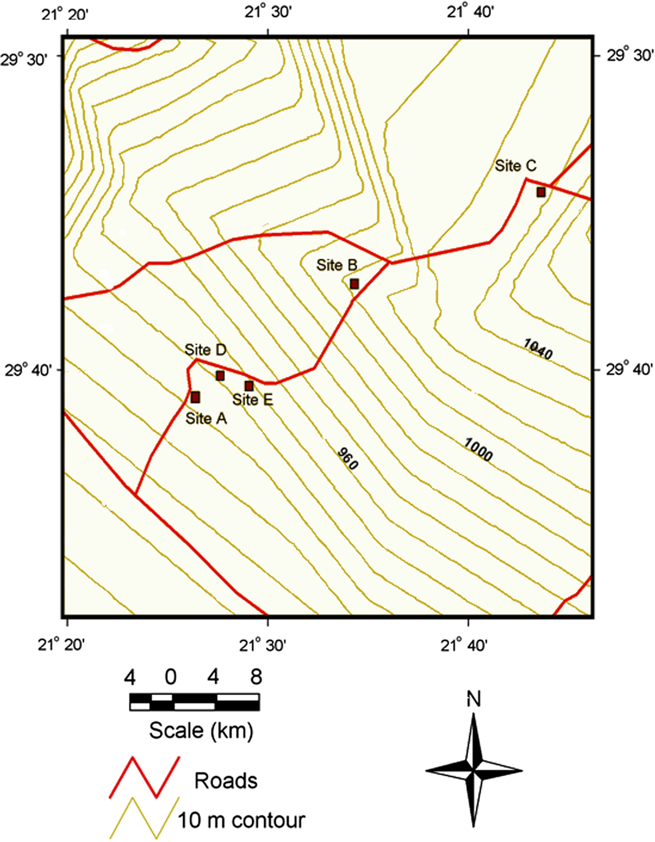
RadarSat (RadarSat-1, superseded by RadarSat-2 launched in 2007), operated by the Canadian Space Agency, was launched in November 1995 and continued functioning until a technical anomaly in April 2013. As with ERS-2, RadarSat was a C-band radar, but it received and transmitted using a horizontal transmit, horizontal receive (HH) polarization. The satellite was in a near-polar, sun-synchronous orbit at an altitude of 798 km and had a revisit rate of 24 days. Two RadarSat images were acquired, one as a standard beam mode 1 (S1) image and the second as a standard beam mode 2 (S2) image, chosen because they most closely resembled the resolution and image scene size of the ERS-2 imagery. The RadarSat imagery was supplied in CEOS format, which were 4-look images, which accounted for their slightly reduced resolution compared with the ERS-2 imagery.

2.2.

Surface Scattering and Surface Roughness

The ability of a material to propagate a pulse of microwave radiation depends on its dielectric constant ( $ε$ ) and the ratio of the pulse velocity in a vacuum to that through the material. When an electromagnetic wave strikes an interface between materials with differing $ε$ , some of the pulse energy is reflected back (surface scattering) and another portion is transmitted through the target material, with the ratio of reflectance to transmittance increasing as the relative difference in the dielectric constants of the two materials increases. If the target material into which the pulse is transmitted is not homogeneous, then the wave will be scattered (volume scattering) as it strikes discontinuities in the target media.

Surface scattering is also affected by the roughness of the target surface (surface roughness) by altering the local incidence angle and hence influencing the direction of the reflected component. Whether the surface roughness plays a role in the amount and structure of the backscatter response or not depends on the wavelength of the incident microwave in relation to the roughness of the surface. Field measurements used to characterize surface roughness of soils are the standard deviation of surface height ( $s$ ) and the surface correlation length ( $l$ ). Provided that the random surface variations are not superimposed on a periodically undulating surface, $s$ can be calculated from a set of surface height measurements made from a reference plane.²³ The correlation length ( $l$ ) is a measure of the minimum distance between two statistically independent surface heights ( $z_{i}$ ) and is essentially a measure of how quickly heights change along a profile. It can be defined as the distance between points for which the autocorrelation function, $ρ (x^{'})$ , is equal to $1 / e$ .²³^–²⁶ The Raleigh criterion states that a surface can be considered smooth if the following condition is met:²³

Eq. (2)

s < \frac{λ}{8 \cos θ},

where

s

is the root mean square (RMS) height (average height variation over the surface, see above),

λ

is the wavelength of the incident microwave, and

θ

is the incidence angle. For the two SAR sensors used, the RMS heights would have to be less than

\sim 0.8 cm

for the target surface to be considered smooth in relation to the wavelength of the incidence wave (radiometrically smooth), allowing the surface roughness to be ignored. The most significant impact of RMS changes will occur as the surface alters from being radiometrically smooth, when coherent scattering away from the sensor dominates, to a radiometrically rough surface when the scattering becomes more diffuse.

2.3.

SAR Backscatter Response

The SAR backscatter response from sparsely vegetated areas is complex but can be modeled by Eq. (3):²⁷

Eq. (3)

σ^{o} = C σ_{veg}^{o} + (1 - C) σ_{veg + soil}^{o} + (1 - C) τ^{2} σ_{soil}^{o},

where

σ^{o}

is the backscatter response (dB),

C

is the fraction of the target area that is covered in vegetation,

σ_{veg}^{o}

is the backscattering due to the vegetation alone,

σ_{veg + soil}^{o}

represents the multiple scattering interactions between vegetation and the soil surface, and

σ_{soil}^{o}

represents the backscatter response from the bare surface. The latter term is qualified by a factor (

τ^{2}

, the square of the vegetation transmissivity) and accounts for the attenuation effect that the vegetation could have on the electromagnetic wave as it is incident on the vegetation and reflected back through it from the soil. In terms of SAR detection of soil moisture, the key factors governing the type of scattering that occurs are as follows:

1. dielectric variation between the atmosphere and the soil surface
2. homogeneity of the soil profile (soil texture)
3. roughness of the soil surface
4. impact of complex scattering from vegetation.

2.4.

Integral Equation Model

The theoretical IEM developed by Fung et al.²⁸ was used to model the bare soil surface backscatter and chosen because of its accuracy under laboratory conditions.²⁹ It has also been shown to provide accurate and meaningful simulation of the SAR backscatter response from bare soil surfaces.²⁸^–³² The IEM model can be broken into two sections depending on the frequency of the incidence wave and the roughness level of the target. If $k s < 3$ , where $k$ is the wave number ( $k = 2 π / λ$ ) and has a value of 1.11 and $s$ is the RMS height, then the surface can be considered small to moderate in terms of surface roughness. Using C band sensors, this criterion is met for a surface with RMS heights $< 2.7 cm$ , making it suitable for most soil surfaces, including those in the Karoo. For surfaces that meet the above criterion, the IEM backscatter response is calculated as

Eq. (4)

σ_{p g}^{o} = \frac{k^{2}}{2} \exp (- 2 k_{z}^{2} s^{2}) \sum_{n = 1}^{N} s^{2 n} {| I_{p q}^{n} |}^{2} \frac{W^{n} (- 2 k_{x}, 0)}{n!},

where

k_{z} = k \cos θ

and

k_{x} = k \sin θ

,

I_{p q}^{n} = {(2 k_{z})}^{n} f_{p q} \exp (- s^{2} k_{z}^{2}) + k_{z}^{n} [F_{p q} (- k_{x}, 0) + F_{p q} (k_{x}, 0)] / 2

, and

p

,

q

indicate the polarization; with

f_{v v} = 2 R_{=} / \cos ϑ

;

f_{h h} = - (2 R_{⊥} / \cos ϑ)

, where

ϑ

is the incidence angle.

R_{=}

and

R_{⊥}

are the Fresnel reflection coefficients, for vertical and horizontal polarization, respectively, at incidence angle

ϑ

.

W^{(n)} (u, v)

is the roughness spectrum of the surface related to the

n

’th power of the surface correlation function

ρ

.

The IEM therefore expresses the backscatter response ( $σ$ ) in terms of (1) SAR frequency, polarization, and incidence angle; (2) soil dielectric constant ( $ε$ ), and (3) RMS height ( $s$ ), correlation function ( $ρ$ ), and the correlation length ( $l$ ). It relies on the assumption adopted here that the bare soil can be exclusively explained as a surface scattering problem with the volume scattering from the soil volume ignored. The IEM model can be successfully calibrated to provide accurate simulations of the backscatter response from natural surfaces using ERS-1, ERS-2, and RadarSat SAR sensors. It is more sensitive to surface roughness variation, especially over smooth surfaces ( $RMS < 5 cm$ ), than it is to soil moisture variation.³⁰^–³³

For the IEM model, it was necessary to determine $ε$ for the soil, achieved by modeling the dielectric constant based on in situ measurements of the soil texture and determined using a modified version of the semiempirical dielectric mixing model,³⁴ which calculates the real part of the dielectric constant based on measurements of soil texture, bulk density $(ρ_{s})$ , and volumetric soil moisture $(θ)$ . Wang and Schmugge³⁴ showed experimentally that the dielectric constant increased at a slower rate with moisture content at the lower end of the soil moisture spectrum, a rate that continues up to a specific level of moisture content termed the transition moisture value, beyond which the rate of increase becomes faster with increasing soil moisture. The transition moisture level $(θ_{t})$ was empirically determined for several types of soils and, following Wang and Schmugge,³⁴ can be calculated using

Eq. (5)

θ_{t} = 0.49 θ_{w p} + 0.165,

where

θ_{w p}

is the permanent wilting point, which is calculated using

Eq. (6)

θ_{w p} = 0.06774 - 0.00064 s \times β_{sand} + 0.00478 \times β_{clay},

where

β_{sand}

and

β_{clay}

are the percentage sand and percentage clay contents of the soil.

For moisture levels below the transition value, the dielectric constant is then calculated as

Eq. (7)

ε = θ ε_{x} + (ϕ - θ) ε_{a} + (1 - ϕ) ε_{r},

where

ε_{a}

and

ε_{r}

are the dielectric constants for air and rock, respectively. A value of 1 for

ε_{a}

and 5.5 for

ε_{r}

was used, as recommended by Wang and Schmugge.³⁴

ϕ

is the porosity of the soil and is calculated as a function of particle density.

ε_{x}

is the dielectric constant of the initially absorbed water, which is calculated using

Eq. (8)

ε_{x} = ε_{i} + (ε_{w} - ε_{i}) \frac{θ}{θ_{t}} γ,

where

ε_{i}

is the dielectric constant of ice, set at 3.2,³⁴ and

ε_{w}

is the real component of the dielectric constant of water, which was calculated using a modified Debye equation. ²⁷

Eq. (9)

ε_{w} = ε_{w \infty} + \frac{ε_{w 0} - ε_{w \infty}}{1 + {(2 π f τ_{w})}^{2}},

where

ε_{w \infty}

is the high-frequency limit of water (set at 4.9, Ref. 27),

ε_{w 0}

is the static dielectric constant of water (set at 80.1, Ref. 27), and

f

is the frequency of the incident wave (Hz). The factor

τ_{w}

is the relaxation time of pure water and is calculated as²⁷

Eq. (10)

2 π τ_{w} (T) = 1.1109 \times 10^{- 10} - 3.824 \times 10^{- 12} T + 6.938 \times 10^{- 14} T^{2} - 5.096 \times 10^{- 16} T^{3},

where

T

is temperature (°C) (set at 20°C).

2.5.

Water Cloud Model

The semiempirical vegetation scattering model used, known as the WCM, was proposed by Attema and Ulaby.³⁵ It is the only existing example of a semiempirical SAR vegetation scattering model and has been extensively assessed in a variety of forms.³⁶ The water cloud approach is based on the proposition that a vegetation layer can be viewed as a cloud of water droplets held in place by the plant components, assuming that the volume scattering is the predominant vegetation scattering mechanism and that the soil-vegetation scattering ( $σ_{veg + soil}^{o}$ ) is ignored. Based on these inputs, an empirical expression of backscatter response from a vegetated surface was described as

Eq. (11)

σ^{o} = C [1 - \exp \frac{- D W h}{\cos θ}] \cos θ + A \exp (B m_{s} - \frac{D W h}{\cos θ}) \cos θ,

where

W

is the vegetation volumetric water content,

h

is the plant height,

m_{s}

is the volumetric soil moisture,

θ

is the incidence angle,

h

is the plant height,

C

and

D

are empirically derived parameters that are related to the scattering from the soil surface, and

A

and

B

are empirical parameters that describe the vegetation scattering. This approach assumes that the vegetation backscatter can be described exclusively in terms of volume scattering, but the inclusion of empirically derived constants means that the effect of vegetation structure is included indirectly. In its original form, the WCM used plant height and water content as the only vegetation inputs.

Prévot et al.³⁶ assessed many additional parameters for suitability for use in the WCM. They chose leaf area index ( $L$ ) as the most suitable indicator since it is correlated with the backscatter response and can be measured remotely. In addition, the use of a single indicator makes model inversion easier. They concluded that $L$ and soil moisture content could be measured through an inversion of a calibrated WCM, provided that two suitable radar configurations were used (X and C bands in this case). Using the same data set, Taconet et al.³⁷ focused on canopy moisture content as an input to the WCM and were able to simulate measured backscatter response to within $\pm 2 dB$ . When this model was inverted, however, they were only able to obtain a rough classification of the soil moisture levels into high, low, and medium. In a later project, Taconet et al.³⁸ used the WCM to derive a correction function for the effect of vegetation using C band measurements with VV polarization. They found that vegetation accounted for a 1-dB change in the backscatter response per $1 kg m^{- 2}$ of canopy moisture and could provide a measure of soil moisture with an accuracy of within $\pm 0.05 {cm}^{3} {cm}^{- 3}$ .

Attema and Ulaby³⁵ suggested three assumptions to be made regarding the structure of the vegetation under consideration: (1) the vegetation is assumed to be represented by a cloud of identical, uniformly distributed water particles, (2) only single scattering need be considered, and (3) the height and density of the cloud are the only factors. Given the unique nature and wide diversity of the vegetation, both in height and structure, being considered within this study, assumptions 1 and 3 may not be applicable. However, the model has been applied in similar circumstances and proven to be useful in understanding the vegetation backscatter response.³⁹^,⁴⁰

2.6.

Field Studies

Field studies were undertaken in the Karoo region of South Africa in March 2001 and April 2002 to measure soil moisture levels, surface roughness, plant density and moisture content, soil texture, and soil bulk density in conjunction with SAR images from the RadarSat and ERS-2 sensors. A $10,000 - {km}^{2}$ site, recorded as an outbreak area of the brown locust for over 45 years,⁴¹ was selected within the Northern Cape province of South Africa near the town of Kenhardt (Fig. 1). In addition to its history, the area was also chosen because of its relatively flat topography, which varies by $< 300 m$ .

Fig. 1

Location of study region in South Africa.

Each of the digital numbers in the SAR imagery represents a measure of the average backscatter response over a unit area ( $\sim 25 \times 25 m$ in the case of ERS-2). This means that any information derived from the imagery, such as a measurement of soil moisture content, will be an average for that area. In the case of the ERS-2 sensor, the value of the backscatter response should be derived from an average of at least 500 pixels in order to obtain an accurate estimate and account for the effect of speckle.⁴² This changes the effective resolution of the imagery, and therefore any measurements made from it, to $\sim 300 \times 300 m$ . Thus, measurements made on the ground must also represent an average value for a $\sim 300 \times 300 - m$ area if an accurate comparison is to be made between image results and ground measurements. To achieve this, a two-tiered field scheme was devised, which consisted of the establishment of large $90,000 - m^{2}$ supersites. Five supersites were established in the northwest section of the study region near Kenhardt. During the 2001 study, three of these sites (supersites A, B, and C) were used and an additional two were included during the 2002 study (supersites D and E) as shown in Fig. 2. Each supersite was selected to include as much of the regional variability in vegetation and surface conditions as possible (Table 2). Choices for site locations were limited to areas that could be easily reached in a challenging environment with difficult access. The centers of all study plots were marked with flagging tape, and global positioning system recordings were taken to ensure that they could be accurately relocated in subsequent field studies and on the geocoded SAR imagery.

Fig. 2

Location of the individual supersites within the study region.

Table 2

General description of each supersite together with a ranking of general veldt condition. The higher the ranking out of 5, the healthier the veldt (grassland) is in terms of vegetation mixture and density.

Supersite	General description	Veldt condition rating (max 5)
A	Equal mixture of grass and shrubs providing an even cover across the area. Elevation $\sim 930 m$	3
B	Situated in a nonperennial pan (a depressed area that may contain standing water during part of the year and usually has internal drainage). The pan areas have distinct surface roughness conditions and vegetation structure. Elevation $\sim 1020 m$	3.5
C	Vegetation dominated by grasses, but the shrubs that are present are larger than on any of the other sites. Some open areas with rocky soils. Elevation $\sim 1030 m$	3
D	Equal mixture of grass and shrubs with large bare areas. Elevation $\sim 940 m$	3
E	Well covered by grasses with some shrubs with a few small open stony areas. Elevation $\sim 940 m$	4

At supersite A, four smaller $25 \times 25 - m$ subplots were established $\sim 300 m$ from each other; at three supersites (B, C, and D), two subplots were established and at supersite E, only one. All the field measurements were then made within each of the subplots. This approach allowed for (1) an assessment of the spatial variability of each of the measured parameters across the supersite, (2) a means of calculating an accurate average result for each parameter over each supersite, and (3) a means of replicating the estimated backscatter response for a given supersite.

Soil moisture measurements were made using volumetric sampling and a capacitance probe (Theta Probe ML #1, Delta-T Devices, Cambridge, UK). Gravimetric soil samples were taken randomly from each of the subplots. The samples were stored in sealed containers, and the moisture content was determined using the double weight method with a drying temperature of 105°C.⁴³ Two cores (5 cm in height and 5 cm in diameter) were also taken randomly from each subregion for bulk density determination and soil particle analysis using a hydrometer method, which allowed for the conversion of the results to a volumetric value.

Within the study region, the vegetation was dominated by dwarf shrubs (chaemaphytes) and grasses (hemicryptophytes), the relative abundance of which are dictated mainly by rainfall and soil.⁴⁴ Shrub species, such as cauliflower ganna (Salsola tuberculata), dominated in sandy areas, and others, such as thorny kapokbush (Eriocephalus spinescens) and three thorn (Rhigozum trichotomum), occurred in more stony areas. The main grasses in the area were small bushman grass (Stipagrostis obtusa) and tall bushman grass (S. ciliata). The presence of grasses and other annuals, such as Pentzia annua and brakspekbos (Zygophyllum simplex), is directly related to seasonal fluctuation in rainfall. Some trees occurred, such as quiver tree (Aloe dichotoma) and bushman poison tree (Euphorbia avasmontana), but these were restricted to either the slopes of kopjes (small hills or rocky outcrops) or to dry river beds, and there were no trees in any of the supersites.

The vegetation on each plot was sampled for moisture content and percent canopy cover. The canopy cover was measured using a line intercept method with a 10-m rope at random locations and orientations.⁴⁵ The distance along the rope that intersected with vegetation was recorded together with the species involved and the average height of the vegetation. The total distance along the 10 m that intersected with vegetation gave a measure of the canopy cover. Two such line intercept measurements were made in each subplot. For moisture content and dry mass, the vegetation from two $0.3 - m^{2}$ quadrats per subregion was harvested from random locations, and moisture content was determined using a double weight method. A measure of soil texture at each of the subsites necessary for the IEM model was obtained using the hydrometer method described by Gee and Bauder,⁴⁶ and the analysis was conducted on the same soil samples gathered for the volumetric soil moisture measurements.

Surface roughness was measured using a 100-cm high-precision profilometer, which consisted of a set of 334 stainless steel pins set into an aluminum box tube through which they could slide. Each pin was 1.5 mm in diameter, and there was an average spacing between each pin of 1.4 mm. At each sampling point, the profilometer was photographed against a reference grid. The photographs were later digitized so that the relative heights between the points could be determined for calculations of the correlation length and RMS. The locations and orientations of each transect for the profilometry were selected with random orientations. The vegetation prevented the measurement of long successive profiles, so 20 profilometer measurements were made in each supersite along a linear transect, and those sections along the transect that intersected with vegetation were omitted. The narrow pins of the profilometer penetrated the loose unconsolidated soil, which may have affected the accuracy of the surface roughness measurements.

3. Results

3.1.

Multitemporal Image Interpretation

The field measurements used for the modeling are summarized in Tables 3 and 4. Figure 3 shows a compilation of three ERS-2 images composed of the September 12, 2000, November 21, 2000, and December 26, 2000, ERS-2 images. The backscatter responses from several distinct image features have been circled and labeled since they consistently returned a distinctive backscatter response. Image area 1 is the backscatter response from a drainage basin containing several distinct pans, dry riverbeds, and kopjes. Site 2 represents what is probably an erosion feature characterized by densely arranged stones on the soil surface. Areas 3 and 4 are the responses from low-lying hills and kopjes. The backscatter responses from these features dominate the results for their zones in each of the images and are examples of areas for which the application of this approach to soil moisture detection would not be appropriate.

Table 3

Estimated surface conditions.

Supersite	RMS (cm)		Correlation length (cm)
Supersite	Estimate	Range	Estimate
A	0.29	0.27 to 0.46	2.41
B	0.20	0.19 to 0.27	7.01
C	0.33	0.21 to 0.35	4.30
D	0.45	0.39 to 0.59	2.90
E	0.34	0.31 to 0.36	4.23

Table 4

Vegetation parameters measured.

Supersite	Canopy cover (%)	Vegetation biomass ( $kg / m^{2}$ )		Vegetation moisture content ( ${cm}^{3} {cm}^{- 3}$ )
Supersite	Canopy cover (%)	Estimate	Range	Estimate	Range
A	18.1	0.49	0.07 to 110	0.10	0.01 to 0.41
B	30.2	1.1	0.28 to 2.71	0.15	0.01 to 0.32
C	26.7	0.33	0.06 to 0.26	0.13	0.01 to 0.07
D	32	0.45	0.22 to 0.74	0.15	0.07 to 0.24
E	26.7	0.34	0.21 to 0.29	0.05	0.01 to 0.09

Fig. 3

Combined ERS-2 images for September 12, 2000, November 21, 2000, and December 26, 2000. The areas circled highlight the backscatter from specific topographic features (see text for details).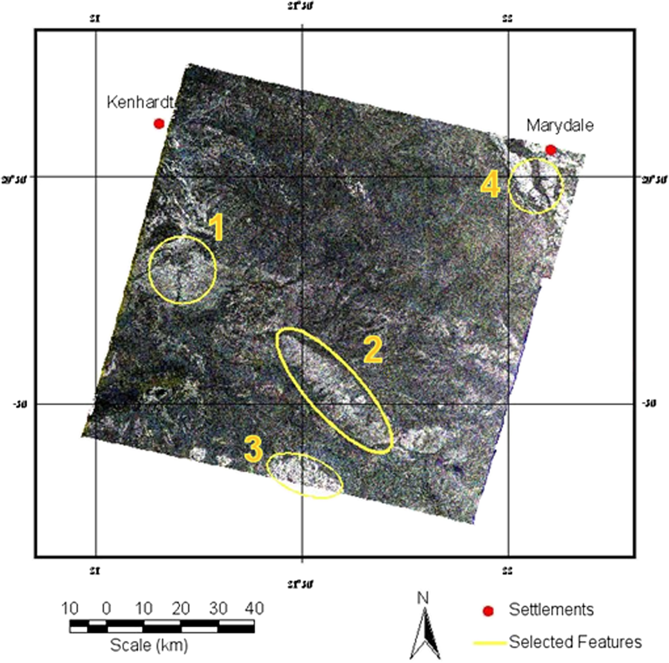

Figures 4 and 5 show eight of the ERS-2 images classified on the basis of the backscatter results. Prior to classification, the images were divided into $\sim 300 - m$ pixels size by taking the average in order to achieve a 95% confidence level in the estimate of the backscatter response. This analysis was limited to these images since they have the same viewing geometry, making surface conditions the only variable.

Fig. 4

Classified ERS-2 images for September 12, 2000, November 21, 2000, December 26, 2000, and March 6, 2001. Images were first resampled into $\sim 300 - m$ pixels prior to classification.

Fig. 5

Classified ERS-2 images for August 28, 2001, October 2, 2001, February 19, 2002, and March 26, 2002. Images were first resampled into $\sim 300 - m$ pixels prior to classification.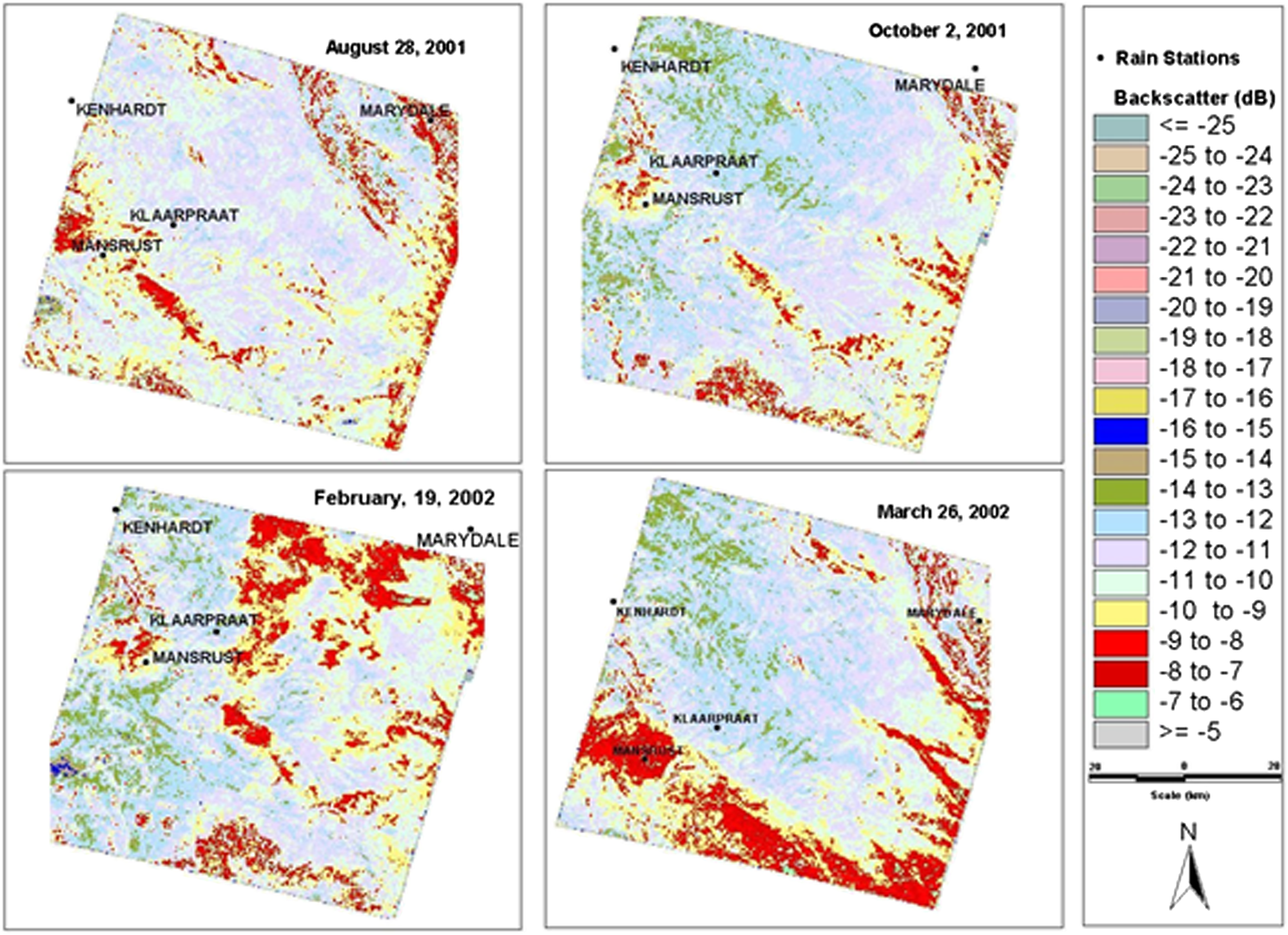

Between September and December 2000, the backscatter response across the region was relatively uniform, which is consistent with reports of no rainfall over this period from nearby rainfall stations. The March 6, 2001, image shows a much lower backscatter response across most of the image, corresponding with the 2001 field study when the region had experienced unusually low rainfall over the previous 6 months, except for the station at Mansrust, which reported a 40.5-mm rainfall event in mid-February. The backscatter response around the Mansrust station in the March 2001 image is higher than that for the areas around the other stations. However, this area is also associated with an area that returns consistently higher backscatter due to its surface conditions. While the drought condition reported for the area would explain the lower overall response, there are other images, such as the September 12, 2000, and August 28, 2001, ones, that were also preceded by several weeks of low rainfall but which did not show low backscatter responses.

The August 28, 2001, image shows a uniform increase in backscatter response across the region in comparison with the March 6, 2001, image. During the intervening period, there were several rainfall events, and each station recorded at least 70 mm of rain. Between the August and October 2001 images, there was only one rainfall event that occurred between 17 and 18 September. While this rainfall event was recorded at each station, the amount recorded varied, with Mansrust having the highest at $\sim 42 mm$ and Marydale and Klaarpraat the lowest with $\sim 13 mm$ each. This rain does not appear to be reflected in the available image results since there was a general decrease in the backscatter response across the entire October 2, 2001, image. Between October 2001 and February 2002, there were at least 14 reported rainfall events with an even distribution across the region. On February 19, 2002, the Marydale station was the only one to report a rainfall event (25 mm). As can be seen on the 19 February image, there is a marked increase in the backscatter response in the northeast corner near the Marydale station, but the response near the other three stations remains similar to that recorded in October 2001.

Comparison of the image and IEM backscatter results for the March 2001 RadarSat and ERS-2 images are shown in Fig. 6 and the results for the April 2002 RadarSat image in Fig. 7. There was some correlation between the IEM and image backscatter results for both the 2001 results ( $r^{2} = 0.78$ ; $P < 0.01$ ) and ( $r^{2} = 0.42$ ; $P = 0.17$ ) for the March 6, 2001, RadarSat and ERS-2 images, respectively. There was little correlation, however, between the IEM and image results in 2002 ( $r^{2} = 0.05$ ; $P = 0.47$ ). In almost all of the subsites in both years, the IEM underestimated the backscatter response. An exception was for supersite A on March 6, 2001, when the ERS-2 image results and those for the IEM model were very similar. The standard error between IEM and image results was 4.7 and 7.1 dB for the March 2001 and April 2002 RadarSat results, respectively, representing errors of $\sim 0.1$ and $0.14 {cm}^{3} {cm}^{- 3}$ in terms of volumetric soil moisture. For the ERS-2 results, the standard error between the model and image was 2.6 dB, which represented an error of $\sim 0.06 {cm}^{3} {cm}^{- 3}$ .

Fig. 6

Integral equation model (IEM) simulation of the backscatter response using the in situ results from the 2001 field study compared with the results from (a) the March 6, 2001, RadarSat image and (b) the March 6, 2001, ERS-2 image. The error bars represent the maximum error due to variation in the in situ measurements of RMS and dielectric constant measurements on the IEM modeling results.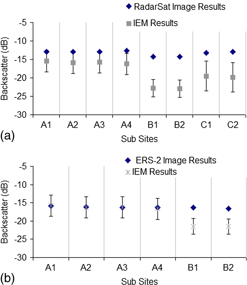

Fig. 7

IEM simulation of the backscatter response using the in situ results from the 2002 field study compared with the results for the April 30, 2002, RadarSat image. The error bars represent the maximum error caused due to variation in in situ measurements of RMS and dielectric constant measurements on the IEM modeling results.

As shown by the IEM results for supersite B in 2001, the model appears to overrespond to the effect of measured in situ variation in surface conditions between supersites. In both of the March 2001 images, the backscatter response from site B is lower than from sites A and C, which may be attributed to the lower RMS at this site. However, the IEM appears to have overresponded to this variation as well. In the 2002 results, the IEM again underestimated the backscatter response in relation to the image results, particularly for supersites B and C, where the model was responding to a measured decrease in the RMS in relation to the other supersites. The measured variability in surface roughness conditions between the supersites is not as evident in the image backscatter as it is in the IEM results.

Even when accounting for the measured variability among the in situ measurements of the RMS and the dielectric constant, the model results were lower than those from the RadarSat image for both years and for site B in the ERS-2 results. Variation in the correlation length has a minimal impact and could not account for the model results. While variation in the dielectric constant could account for the variation, there is no evidence based on the field measurements that the calculated dielectric constants were not accurate. However, an inversion of the IEM for the dielectric constant, using the image backscatter as input along with the in situ measurements of surface roughness, showed that resulting dielectric constants were unrealistically high for the conditions encountered in the field. The two remaining variable factors are the shape of the autocorrelation function and the estimates of the RMS height. As seen in Fig. 8, for the 2001 RadarSat image, changing the shape of the autocorrelation function to Gaussian improved the IEM simulation for supersite A but had little impact on the results for sites B and C. These inconsistent results were also obtained for the 2002 RadarSat results and the 2001 ERS-2 image.

Fig. 8

IEM results using a Gaussian shaped correlation function with the 2001 RadarSat input data compared with 2001 RadarSat image results for each subsite. The error bars represent the maximum error caused due to variation in RMS and dielectric constant measurements.

3.2.

Water Cloud Model

Analysis was restricted to the use of the March 6, 2001, ERS-2 and the two RadarSat images (March 6, 2001, and April 30, 2002) since these were the only dates for which field data on vegetation conditions were available. Before applying the model, it was necessary to make the assumption that the vegetation over each of the study sites was similar in structure and that any variation between plots was attributable to measurable in situ factors. Unfortunately in situ data from the Karoo for parameters such as leaf area index, leaf surface area, and density were not available due to difficulty in measuring them in the field. Plant height was recorded as part of the line intercept study, but the variation caused by the wide variety of plant types made it an impractical model input. However, the following potential vegetation inputs were available:

1. plant biomass per unit area—measured from the vegetation quadrats
2. plant moisture per unit area—measured from the vegetation quadrats
3. percent canopy cover—measured from the line intercept.

A linear regression analysis was conducted between the SAR image backscatter from each of the field sites and the above three field parameters, based on which plant biomass and plant moisture were chosen for evaluation as an input into the WCM, as they were the only variables with values of $R^{2}$ consistently $> 0.50$ . It should be noted that soil moisture variability was not included as part of this regression analysis since it was not possible to separate its effects from that of the vegetation. If moisture variability is a factor, then the significance of any one of these factors may be underrepresented using this analysis method.

If the soil-vegetation scattering ( $σ_{veg + soil}^{o}$ ) component is ignored, Eq. (3) can be simplified to

Eq. (12)

σ^{o} = σ_{veg}^{o} + τ^{2} σ_{soil}^{o} .

In its original form, the WCM relies on a generalized linear relationship between soil moisture and backscatter from the soil surface in order to derive values for parameters $C$ and $D$ . This approach ignores the significance of the other variables, such as surface roughness and soil texture, which have already been shown to be significant factors in the backscatter response. To avoid this problem, the IEM was used to model the bare surface soil component by first assuming that the ratio between the image backscatter results ( $σ_{image}^{o}$ ) and IEM ( $σ_{iem}^{o}$ ) simulations results is equal to the square of the vegetation transmissivity ( $τ^{2}$ ). In optical terms, the transmissivity is equivalent to transmittance and is the ratio between transmitted and incident power.

The vegetation constant $B$ can then be calculated from³⁹

Eq. (13)

\frac{σ_{image}}{σ_{iem}} = τ^{2} = \exp (\frac{- 2 B X_{y}}{\cos θ}),

where

X_{y}

is the vegetation input parameter, moisture (

m_{v}

), or biomass (

b_{v}

).

The vegetation scattering $σ_{veg}^{o}$ is then calculated, following Prevot et al.,⁴⁷ using

Eq. (14)

σ_{veg}^{o} = A X_{y} \cos θ (1 - τ^{2}) .

Under this interpretation, the vegetation parameter $A$ can be seen as a vegetation density parameter and $B$ as measure of the vegetation attenuation. Two forms of the WCM were parameterized separately using both vegetation moisture and vegetation biomass as the sole input. Since polarization is a factor and not explicitly included in the derivation of the model, parameters would have to be unique for each of the two sensors.

The water cloud results were then assessed against the 2001 ERS-2 and RadarSat backscatter results and, in the case of the RadarSat configuration, independently assessed by using the 2002 in situ and image data using both parameters. The regression coefficient (Fig. 9) between the WCM simulations and the 2001 image results is reduced in comparison with the value for a direct regression between the vegetation parameters and image results, except in the case of the RadarSat image when biomass was used as a model input. For the RadarSat results, the regression between water cloud results when vegetation moisture was used is also lower than between the bare surface IEM results and the image. In the case of the ERS-2 results, the regression is approximately the same using the WCM as was found for the bare surface IEM results. For the ERS-2 results, the application of the WCM only resulted in a slight improvement in the standard error from 2.9 dB for the IEM alone to 1.51 and 2.05 dB with use of vegetation moisture and biomass, respectively. In the case of the RadarSat results, there was a much larger reduction in the standard error from 4.7 dB from the IEM alone to 0.64 and 0.34 dB with use of vegetation moisture and biomass, respectively.

Fig. 9

Scatter plots of measured backscatter response from the ERS-2 and RadarSat synthetic aperture radar sensors and estimates generated by the water cloud model using vegetation moisture [(a) and (c)] and vegetation biomass [(b) and (d)] as model inputs. Model parameters A and B were generated using the 2001 data set.

Figure 10 shows the modeled results for each of the subsites. The addition of the WCM did not substantially improve the overall modeling results for the ERS-2 image. When vegetation moisture was used, the WCM caused the backscatter response to be overestimated for supersite A. For site B, the model did improve the net comparison but was not able to fully account for the lower IEM results. In the case of the RadarSat results, the WCM accounted for almost all of the variation between the IEM and image results using either of the vegetation inputs, including the results for subsite B where the largest variation occurred. For some plots, such as supersite C, the WCM overcompensated, resulting in an overestimation of the backscatter response. Overall, however, the application of the WCM was able to account for variation both within and between supersites based solely on in situ measurements of vegetation.

Fig. 10

Modeled backscatter from the water cloud model for each subsite along with the image results and bare surface IEM model results for the March 6, 2001, ERS-2 results [(a) and (b)] and the March 6, 2001, RadarSat results [(c) and (d)].

When the model was used in forward application with the 2002 in situ results and the 2002 RadarSat image, there was once again no improvement in the correlation between model and image results (data not shown). Both versions of the model did, however, provide a net improvement compared with the original IEM in the standard error and could account for up to 60% of the variation.

4. Discussion

An explicit calibration of the IEM model based on the in situ measurements of the surface roughness conditions in the Karoo showed that theoretically the model can provide estimates of the volumetric soil moisture content with an accuracy of approximately $\pm 0.06 {cm}^{3} {cm}^{- 3}$ if RMS (average height variation over the surface) is treated as the only variable. The relatively smooth conditions of the measured soil surfaces in the Karoo meant that slight variations of RMS over time and location can have dominant impacts on the backscatter response. Prior knowledge of the surface roughness over the regions would therefore be necessary before the model could be extrapolated for use in areas beyond those used in this study. A direct assessment of the IEM capabilities by comparison with images from the ERS-2 SAR sensor found that the theoretical level of accuracy is achievable, but due to a series of ERS-2 imager failures, the analysis was limited and this result needs confirmation. A more comprehensive assessment using the RadarSat SAR sensor indicated that a significantly larger error of $\pm 0.14 {cm}^{3} {cm}^{- 3}$ in estimates of volumetric soil moisture could be expected.

The IEM modeling process showed that some portion of the increased level of variability encountered in the RadarSat and ERS-2 assessments could be attributed to errors in the in situ measurement of the RMS and possible impact of additional factors such as vegetation, the amounts of which could potentially have an impact on the backscatter response. A further indication that vegetation over the study sites was contributing to the SAR backscatter response was provided by the parameterization and application of modified versions of the WCM using vegetation biomass and vegetation moisture as inputs. A sensitivity study of the resulting vegetation scattering models found that there was a positive relationship between increasing backscatter and both vegetation biomass and vegetation moisture. For the RadarSat imagery, the WCM was able to account for up to 80% of the variability between IEM and image results for some sites.

The sensitivity of the IEM to slight changes in RMS over the Karoo along with the demonstrated role of vegetation biomass and moisture means that concurrent information on these factors is needed to derive accurate quantitative estimates of volumetric soil moisture using the sensors and methodology outlined here. Currently, there is no readily available means of acquiring this type of spatial information, which limits the potential use of the IEM model alone for the Karoo since there is no means of assessing accuracy if the model is extrapolated to areas where there is no prior knowledge of the surface roughness and vegetation conditions.

Directly relating the results of this research to the needs of brown locust researchers and controllers is currently difficult due to the lack of quantitative information on the moisture dynamics of brown locust egg development. Specific information on the egg moisture requirements measured in terms such as volumetric soil moisture is necessary in order to assess the applicability of tools such as SAR imagery. Based on the moisture requirements for the egg development of the Australian plague locust, the SAR used in this study can theoretically provide soil moisture measurements with an accuracy that is meaningful to locust forecasters. The level of error in the SAR estimates of soil moisture that was directly identified as part of this study means that further research is necessary to identify means of accounting for factors such as vegetation and surface roughness.

Two key points that require further investigation are methods of assessing both surface roughness and vegetation in terms that are relevant to SAR backscatter from space-borne sensors. For surface roughness, the possible errors that may have been introduced by the profilometer could be avoided through the use of a laser profilometer such as the one described by Davidson et al.,⁴⁸ which would not require physical disruption of the soil surface. Lu and Meyer⁴⁹ used repeat-pass ERS-1 SAR imagery to separate backscatter due to surface roughness from backscatter changes assumed to be due to a rainfall event and so successfully estimated soil moisture at a site in Mexico. There is also the possibility of assessing the surface roughness directly from SAR using

• Multiangular imagery from sensors such as RadarSat, ENVISAT, and RadarSat-2. Since the incidence angle has a direct impact on the backscatter response, the variation between two images can be used as a measure of surface roughness.⁵⁰^,⁵¹ Also, at higher incidence angles ( $> 40 \deg$ ), the effect of surface roughness from bare soils becomes the dominant factor in backscatter responses,²⁷^,⁵²^,⁵³ which can provide a means of classifying the target area into roughness types. In addition, SAR interferometry has also been shown to have the capability of assessing surface roughness.⁵⁴
• The European Space Agency’s ENVISAT sensor with its dual channel capabilities must also be assessed, particularly the cross-polar vertical-horizontal (VH) capabilities, which have been shown to have a distinct surface roughness response.²⁸

Any additional studies in the Karoo will need to attempt to measure in situ vegetation parameters that could be used in a theoretical vegetation scattering model. Given the mixed vegetation in the Karoo, a multilayered approach would be required in which distinct vegetation types are grouped and assessed separately. For examples of the types of parameters needed, see Chiu and Sarabandi⁵⁵ and Macelloni et al.³¹

Another area that has received little attention is the use of ancillary imagery in the assessment of the SAR response to vegetation. Novel optical indices, such as the global vegetation moisture index (GVMI), have been developed specifically to assess vegetation moisture⁵⁶ and may prove useful for assessing the impact of vegetation on the SAR backscatter response. Also, higher-resolution optical imagery from platforms such as Landsat may also provide more meaningful results since they provide a resolution closer to that of the SAR imagery.

The future applicability of SAR imagery in brown locust forecasting will depend on the technical feasibility of acquiring imagery on a spatial and temporal scale that is useful for forecasters. Even with the more advanced SAR sensors aboard ENVISAT and RadarSat-2, it is unlikely that high-resolution images such as the ones used in this study could be acquired on a regular basis for the entire brown locust outbreak area due to the limited scene size. Other SAR image producers such as the RadarSat ScanSar and ENVISAT wide swath images should be the focus of future research for soil moisture detection in the Karoo since they offer a more realistic means of acquiring imagery on a more meaningful repeat cycle and image scale. Once achieved, such a system could provide short-term forecasts in conjunction with longer-term forecasts based, for instance, on sea surface temperatures.⁵⁷ Future work on the biology of the brown locust needs to define soil moisture requirements in terms of soil moisture availability, rather than using rainfall alone, so that the required sensitivity of instruments such as SAR for soil moisture monitoring can be more clearly defined.

Acknowledgments

A studentship for W.T.S.C. at the Natural Resources Institute was funded by the Higher Education Funding Council for England. Additional funding was received from Natural Resources International through a Natural Resources International 2001 Postgraduate Study/International Travel Fellowship. Complimentary SAR was provided by the European Space Agency and at a reduced rate from RadarSat International. We thank Dr. David Archer and Dr. Chris Sear for their advice and assistance and collaborators in South Africa, including Margaret Kieser and Roger Price from the South African Plant Protection Research Institute (ARC-PPRI); Annecke Thakrah from the ARC Institute for Soil, Climate and Water; and Seppie Esterhuysen from the Northern Cape Province agriculture extension office. Staff at the ARC Range and Forage Institute in Upington conducted some of the laboratory work. We thank the two anonymous referees for their constructive inputs, which led to improvements to an earlier draft.

References

1.

B. P. Uvarov, Grasshoppers and Locusts. A Handbook of General Acridology, Cambridge University Press, Cambridge (1966). Google Scholar

2.

B. P. Uvarov, Grasshoppers and Locusts. A Handbook of General Acridology, Centre for Overseas Pest Research, London (1977). Google Scholar

3.

The Locust and Grasshopper Agricultural Manual, Centre for Overseas Pest Research, London (1982). Google Scholar

4.

L. V. Bennett, “The development and termination of the 1968 plague of the desert locust, Schistocerca gregaria (Forskål) (Orthoptera: Acrididae),” Bull. Entomol. Res., 66 511 –552 (1976). http://dx.doi.org/10.1017/S000748530000691X BEREA2 0007-4853 Google Scholar

5.

A. C. Saraiva, “Plague locusts—Oedaleus senegalensis (Krauss) and Schistocerca gregaria (Forskål) in the Cape Verde Islands,” Estudos Agron., 3 61 –89 (1962). Google Scholar

6.

L. D. C. FishpoolR. A. Cheke, “Protracted eclosion and viability of Oedaleus senegalensis (Krauss) eggs (Orthoptera,Acrididae),” Entomol. Monthly Mag., 119 215 –219 (1983). ENMMAT 0013-8908 Google Scholar

7.

J. U. HielkemaJ. RoffeyC. J. Tucker, “Assessment of ecological conditions associated with the 1980/81 desert locust plague upsurge in West Africa using environmental satellite data,” Int. J. Remote Sens., 7 1609 –1622 (1986). http://dx.doi.org/10.1080/01431168608948956 IJSEDK 0143-1161 Google Scholar

8.

K. Cressman, “The use of new technologies in desert locust early warning,” Outlooks Pest Manage., 19 55 –59 (2008). http://dx.doi.org/10.1564/19apr03 OPMUB8 1743-1026 Google Scholar

9.

J.-F. Pekelet al., “Development and application of multi-temporal colorimetric transformation to monitor vegetation in the desert locust habitat,” IEEE J. Sel. Topics Appl. Earth Obs. Remote Sens., 4 318 –326 (2011). http://dx.doi.org/10.1109/JSTARS.2010.2052591 1939-1404 Google Scholar

10.

P. Ceccatoet al., “The desert locust upsurge in West Africa (2003–2005): information on desert locust early warning system and the prospects for seasonal climate forecasting,” Int. J. Pest Manage., 53 7 –13 (2007). http://dx.doi.org/10.1080/09670870600968826 IPEMEH 0967-0874 Google Scholar

11.

J. C. FaureS. J. Marais, “The control of Locustana pardalina in its outbreak centres,” in Proc. of the 4th Int. Locust Conf., (1936). Google Scholar

12.

H. D. Brown, “Locust—a new threat,” Research Highlights, 1987: Plant Production, 153 –156 Department of Agriculture Water Supply, Government Printer, Pretoria, Republic of South Africa (1987). Google Scholar

13.

M. E. KieserA. ThackrahJ. Rosenberg, “Changes in the outbreak region of the brown locust,” (2002) http://gadi.agric.za/articles/Kieser_M/kieser_vol4_2002_locust.php Google Scholar

14.

A. Lea, “Recent outbreaks of the brown locust, Locustana pardalina (Walker), with special reference to the influence of rainfall,” J. Entomol. Soc. South Africa, 21 162 –213 (1958). Google Scholar

15.

R. E. PriceH. D. Brown, “A century of locust control in South Africa,” in Workshop on Research Priorities for Migrant Pests of Agriculture in Southern Africa, 24–26 March 1999, 37 –49 (2000). Google Scholar

16.

Locust Handbook, 2nd ed.Overseas Development Natural Resources Institute, London (1988). Google Scholar

17.

J. J. Matthée, “The structure and physiology of the egg of Locustana pardalina (Walk),” Union of S. Africa Dept. Agric. Forest Sci. Bull., 316 1 –83 (1951). Google Scholar

18.

C. Smit, Field Observations on the Brown Locust in an Outbreak Area, Department of Agriculture and Forestry, South African Government, Pretoria (1939). Google Scholar

19.

R. E. Price, “The life cycle of the brown locust, with reference to egg viability,” in Proc. of the Locust Symposium, 27 –40 (1988). Google Scholar

20.

D. HunterT. Deveson, “Forecasting and management of migratory pests in Australia,” Entomol. Sin., 9 13 –25 (2002). Google Scholar

21.

F. T. UlabyP. P. BatlivalaM. C. Dobson, “Microwave backscatter dependence of surface roughness, soil moisture, and soil texture, Part 1—bare soil,” IEEE Trans. Geosci. Remote Sens., 16 286 –295 (1978). IGRSD2 0196-2892 Google Scholar

22.

Y. DuF. T. UlabyM. C. Dobson, “Sensitivity to soil moisture by active and passive microwave sensors,” IEEE Trans. Geosci. Remote Sens., 38 105 –114 (2000). http://dx.doi.org/10.1109/36.823905 IGRSD2 0196-2892 Google Scholar

23.

Microwave Remote Sensing: Active and Passive, Volume II: Radar Remote Sensing and Surface Scattering and Emission Theory, Addison-Wesley, Reading, Massachusetts (1982). Google Scholar

24.

R. J. Wanget al., “The SIR-B observations of microwave backscatter dependence on soil moisture, surface roughness, and vegetation covers,” IEEE Trans. Geosci. Remote Sens., GE-24 510 –516 (1986). http://dx.doi.org/10.1109/TGRS.1986.289665 IGRSD2 0196-2892 Google Scholar

25.

P. Bertuzziet al., “The use of microwave backscatter model for retrieving soil moisture over bare soil,” Int. J. Remote Sens., 13 2653 –2668 (1992). http://dx.doi.org/10.1080/01431169208904070 IJSEDK 0143-1161 Google Scholar

26.

Y. OhY. C. Kay, “Condition for precise measurement of soil surface roughness,” IEEE Trans. Geosci. Remote Sens., 36 691 –695 (1998). http://dx.doi.org/10.1109/36.662751 IGRSD2 0196-2892 Google Scholar

27.

Microwave Remote Sensing: Active and Passive, Volume III: From Theory to Applications, Addison-Wesley, Reading, Massachusetts (1986). Google Scholar

28.

A. K. FungZ. LiK. S. Chen, “Backscatter from a randomly rough dielectric surface,” IEEE Trans. Geosci. Remote Sens., 30 356 –369 (1992). http://dx.doi.org/10.1109/36.134085 IGRSD2 0196-2892 Google Scholar

29.

A. K. Fung, Microwave Scattering and Emission Models and Their Application, Artech House, Norwood, Massachusetts (1994). Google Scholar

30.

E. Alteseet al., “Retrieving soil moisture over bare soil from ERS 1 synthetic aperture radar data: sensitivity analysis based on a theoretical surface scattering model and field data,” Water Resour. Res., 32 653 –661 (1996). http://dx.doi.org/10.1029/95WR03638 WRERAQ 0043-1397 Google Scholar

31.

G. Macelloniet al., “The relationship between the backscattering coefficient and the biomass of narrow and broad leaf crops,” IEEE Trans. Geosci. Remote Sens., 39 873 –884 (2001). http://dx.doi.org/10.1109/36.917914 IGRSD2 0196-2892 Google Scholar

32.

K. TanseyA. C. Millington, “Investigating the potential for soil moisture and surface roughness monitoring in drylands using ERS SAR data,” Int. J. Remote Sens., 22 2129 –2149 (2001). IJSEDK 0143-1161 Google Scholar

33.

G. F. BiftuT. Y. Gan, “Retrieving near-surface soil moisture from Radarsat SAR data,” Water Resour. Res., 35 1569 –1579 (1999). http://dx.doi.org/10.1029/1998WR900120 WRERAQ 0043-1397 Google Scholar

34.

R. J. WangT. J. Schmugge, “An empirical model for the complex dielectric permittivity of soils as a function of water content,” IEEE Trans. Geosci. Remote Sens., 18 288 –295 (1983). IGRSD2 0196-2892 Google Scholar

35.

E. P. AttemaF. T. Ulaby, “Vegetation modelled as a water cloud,” Radio Sci., 13 357 –364 (1978). http://dx.doi.org/10.1029/RS013i002p00357 RASCAD 0048-6604 Google Scholar

36.

L. PrévotI. ChampionG. Guyot, “Estimating surface soil moisture and leaf area index of a wheat canopy using a dual frequency (C and X bands) scatterometer,” Remote Sens. Environ., 46 331 –339 (1993). http://dx.doi.org/10.1016/0034-4257(93)90053-Z RSEEA7 0034-4257 Google Scholar

37.

O. Taconetet al., “Estimation of soil and crop parameters for wheat from airborne radar backscattering data in C and X bands,” Remote Sens. Environ., 50 287 –294 (1994). http://dx.doi.org/10.1016/0034-4257(94)90078-7 RSEEA7 0034-4257 Google Scholar

38.

O. Taconetet al., “Taking into account vegetation effects to estimate soil moisture from C-band radar measurements,” Remote Sens. Environ., 56 52 –56 (1996). http://dx.doi.org/10.1016/0034-4257(95)00212-X RSEEA7 0034-4257 Google Scholar

39.

T. SvorayM. Shoshany, “SAR-based estimation of areal above ground biomass (AAB) of herbaceous vegetation in the semi-arid zone: a modification of the water cloud model,” Int. J. Remote Sens., 23 4089 –4100 (2002). http://dx.doi.org/10.1080/01431160110115924 IJSEDK 0143-1161 Google Scholar

40.

R. BindlishA. P. Barros, “Multifrequency soil moisture inversion from SAR measurements with the use of IEM,” Remote Sens. Environ., 71 67 –88 (2000). http://dx.doi.org/10.1016/S0034-4257(99)00065-6 RSEEA7 0034-4257 Google Scholar

41.

M. E. Keiser, , Personal Communication (25 March 1999).M. E. Keiser, , Personal Communication (25 March 1999).

42.

H. Lauret al., “Derivation of the backscattering coefficient σo in ESA ERS SAR Pri products,” in Proc. of the Second International Workshop on ERS Applications, 139 (1998). Google Scholar

43.

W. H. Gardner, “Water content: gravimetry with oven drying,” Methods of Soil Analysis: Part 1—Physical and Mineralogical Methods, 503 –507 2nd ed.American Society of Agronomy Inc. & Soil Science Society of America Inc., Wisconsin (1986). Google Scholar

44.

W. R. J. DeanS. J. Milton, The Karoo: Ecological Patterns and Processes, Cambridge University Press, Cambridge (1999). Google Scholar

45.

M. KentP. Coker, Vegetation Description and Analysis: A Practical Approach, Belhaven, London (1992). Google Scholar

46.

G. W. GeeJ. W. Bauder, “Particle-size analysis,” Methods of Soil Analysis: Part 1—Physical and Mineralogical Methods, 383 –411 2nd ed.American Society of Agronomy Inc. & Soil Science Society of America Inc., Wisconsin (1986). Google Scholar

47.

L. Prevotet al., “Estimating the characteristics of vegetation canopies with airborne radar measurements,” Int. J. Remote Sens., 14 2803 –2818 (1993). http://dx.doi.org/10.1080/01431169308904310 IJSEDK 0143-1161 Google Scholar

48.

M. Davidsonet al., “On the characterization of agricultural soil roughness for radar remote sensing studies,” IEEE Trans. Geosci. Remote Sens., 38 630 –640 (2000). http://dx.doi.org/10.1109/36.841993 IGRSD2 0196-2892 Google Scholar

49.

Z. LuD. J. Meyer, “Study of high SAR backscattering caused by an increase of soil moisture over a sparsely vegetated area: implications for characteristics of backscattering,” Int. J. Remote Sens., 23 1063 –1074 (2002). http://dx.doi.org/10.1080/01431160110040035 IJSEDK 0143-1161 Google Scholar

50.

M. AutretR. DernardD. Vidal-Madjar, “Theoretical study of the sensitivity of microwave backscattering coefficient to the soil surface parameters,” Int. J. Remote Sens., 10 171 –179 (1989). http://dx.doi.org/10.1080/01431168908903854 IJSEDK 0143-1161 Google Scholar

51.

B. Colpitts, “The integral equation model and surface roughness signatures in soil moisture and tillage type determination,” IEEE Trans. Geosci. Remote Sens., 36 833 –837 (1998). http://dx.doi.org/10.1109/36.673676 IGRSD2 0196-2892 Google Scholar

52.

N. Baghdadiet al., “Potential of ERS and RadarSat data for surface roughness monitoring over bare agricultural fields: application to catchment in Northern France,” Int. J. Remote Sens., 23 3427 –3442 (2002). http://dx.doi.org/10.1080/01431160110110974 IJSEDK 0143-1161 Google Scholar

53.

N. Baghdadiet al., “An empirical calibration of the integral equation model based on SAR data, soil moisture and surface roughness measurement over bare soils,” Int. J. Remote Sens., 23 4325 –4340 (2002). http://dx.doi.org/10.1080/01431160110107671 IJSEDK 0143-1161 Google Scholar

54.

U. Wegmuller, “Soil moisture monitoring with ERS SAR interferometry,” in Proc. of the Third ERS Scientific Symp., (1997). Google Scholar

55.

T. ChiuK. Sarabandi, “Electromagnetic scattering from short branching vegetation,” IEEE Trans. Geosci. Remote Sens., 38 911 –925 (2000). http://dx.doi.org/10.1109/36.841974 IGRSD2 0196-2892 Google Scholar

56.

P. CeccatoS. FlasseJ.-M. Gregoire, “Designing a spectral index to estimate vegetation water content from remote sensing data. Part 2. Validation and applications,” Remote Sens. Environ., 82 198 –207 (2002). http://dx.doi.org/10.1016/S0034-4257(02)00036-6 RSEEA7 0034-4257 Google Scholar

57.

M. Toddet al., “Brown locust outbreaks and climate variability in Southern Africa,” J. Appl. Ecol., 39 31 –42 (2002). http://dx.doi.org/10.1046/j.1365-2664.2002.00691.x JAPEAI 0021-8901 Google Scholar

Biography

William T. S. Crooks has a BSc in agricultural science with a specialization in soil science from University of Guelph, Canada (1993), an MSc in the same speciality from Dalhousie University and Nova Scotia Agricultural College, Halifax, Canada (1997), and an advanced degree certificate in geographical information systems (GIS) from the College of Geographical Sciences, Lawrencetown, Canada. He obtained his PhD at University of Greenwich in 2003 and is now based at the Scotland’s Rural College, Ayr, Scotland.

Robert A. Cheke graduated with a BSc in zoology from the University of St. Andrews, Scotland, in 1970 and a PhD at the University of Leeds, England, in 1974. He joined the Centre for Overseas Pest Research (now the Natural Resources Institute of the University of Greenwich) in 1976, where he has worked on grasshoppers, locusts, blackfly vectors of onchocerciasis, quelea birds, and other pests in Africa. He was appointed professor of tropical zoology in 1997.

CC BY: © The Authors. Published by SPIE under a Creative Commons Attribution 4.0 Unported License. Distribution or reproduction of this work in whole or in part requires full attribution of the original publication, including its DOI.

Citation Download Citation

William T. Crooks and Robert A. Cheke "Soil moisture assessments for brown locust Locustana pardalina breeding potential using synthetic aperture radar," Journal of Applied Remote Sensing 8(1), 084898 (18 March 2014). https://doi.org/10.1117/1.JRS.8.084898

Published: 18 March 2014

Access the abstract

JOURNAL ARTICLE
23 PAGES

DOWNLOAD PAPER SAVE TO MY LIBRARY

GET CITATION

CITATIONS

Cited by 20 scholarly publications.

Explore citations on Lens.org

KEYWORDS

Vegetation

Soil science

Backscatter

Synthetic aperture radar

Surface roughness

Scattering

Dielectrics

1.

Introduction

Eq. (1)

2.

Methods

2.1.

Satellite Imagery

Table 1

2.2.

Surface Scattering and Surface Roughness

Eq. (2)

2.3.

SAR Backscatter Response

Eq. (3)

2.4.

Integral Equation Model

Eq. (4)

Eq. (5)

Eq. (6)

Eq. (7)

Eq. (8)

Eq. (9)

Eq. (10)

2.5.

Water Cloud Model

Eq. (11)

2.6.

Field Studies

Fig. 1

Fig. 2

Table 2

3.

Results

3.1.

Multitemporal Image Interpretation

Table 3

Table 4

Fig. 3

Fig. 4

Fig. 5

Fig. 6

Fig. 7

Fig. 8

3.2.

Water Cloud Model

Eq. (12)

Eq. (13)

Eq. (14)

Fig. 9

Fig. 10

4.

Discussion

Acknowledgments

References

Biography

Show All Keywords

Keywords/Phrases

Search In:

Publication Years