1.

Introduction

Remote sensing is an effective technology to extract and map spatially explicit information of land use and cover at different scales.^1,2 Forest cover maps are one of the products made using remotely sensed data and are essential for forest management, habitat monitoring, and biodiversity analysis.^3–6 General-purpose land cover maps developed at national and global scales usually describe forest information at a coarse level. For example, the National Land Cover Database (NLCD)⁷ for the United States contains three forest types: deciduous, evergreen, and mixed forests, a level-II classification defined by the United State Geological Survey (USGS).⁸ For the purposes of intensive forest management, habitat characterization, and forest health monitoring, it is essential to obtain more detailed forest information than the USGS (or Anderson) level-II classification can provide.^9–11

The major challenge in land use or forest classification is to increase classification detail with satisfactory accuracy.^12–14 This is because forest classification can theoretically be made at any level but classification accuracy decreases with increasing classification detail. Fine-level forest cover maps with low classification accuracy are no better than coarse-level forest cover maps with high classification accuracy though different forest management activities may require different forest cover maps. A three-forest-class (or Anderson’s level-II) land cover map works well for national-scale forest assessment, but is insufficient for complex forest management at the state level, such as in Indiana where 95% of forests are deciduous.¹⁵ In this region, distinct deciduous hardwood forest types exist, requiring differing silvicultural regimes for management and maintenance.^10,16 However, detailed classification of hardwood forests is difficult due to the similarities in spectral reflectance, canopy structure, and spatial mixture of hardwood tree species.¹⁷

There is a clear need for a quality forest cover map in Indiana to assess the habitat availability for bat species that are at risk from white-nose syndrome.¹⁸ For example, the Indiana bat (Myotis sodalis) is listed as an endangered species by the U.S. Fish and Wildlife Service as well as the International Union for Conservation of Nature.¹⁹ Populations of Indiana bats have declined $>50\%$ from 1960 to 2001²⁰ and are under considerable threat of increased declines due to white-nose syndrome.²¹ During the summer, Indiana bats mainly use hardwood and hardwood-pine forests²² and a quality forest cover map can assist in modeling current and future bat habitat.²³

There are several existing forest cover maps that contain more than three forest types at national or state scales. The Forest Cover Types map produced by the National Atlas of the United States²⁴ provides an alternative resource for obtaining a forest cover map in Indiana. This dataset was created based on advanced very high resolution radiometer and Landsat Thematic Mapper (TM) imagery acquired in 1991 and includes 25 types of forests with a 1-km spatial resolution. The classifications of hardwood forests, however, do not separate maple (Acer sp.) from mixed hardwood tree species groups despite the fact that maple is one of the most dominant tree genera in Indiana. Furthermore, there is no accuracy assessment information associated with the metadata. The Indiana Gap Analysis Project has also produced a land cover map.²⁵ The development of this land cover map focused upon habitat attributes but did not consider subclasses of hardwood forests. The overall accuracy of this map was just 70.98%. However, for the assessment of land use and land cover mapping, the USGS proposed a recommendation of minimum accuracy of 85%.⁸ For application in landscape quantification, a classification accuracy of $>85\%$ is necessary.¹³ Although there is no specific accuracy requirement for the purpose of forest managements and habitat delineation, our objective was to develop a forest cover map with 85% or better classification accuracy. Existing land cover maps were not satisfactory in terms of classification details and accuracy; therefore, it was necessary to develop a more accurate and more detailed forest cover map to meet the needs of various spatial analyses, such as wildlife habitat simulations.

The algorithms of image data classification to derive a forest cover map generally include supervised and unsupervised approaches.²⁶ Supervised classifications require training a dataset to predefine the statistical parameters (such as maximum likelihood) or nonparametric statistical learning functions (such as neural network and support vector machine).^27,28 Unsupervised classifications (such as ISODATA and K-means clustering) generate spectral clusters based on the statistical information of the remote sensing imagery.^29,30 Supervised and unsupervised classifications each have their own strengths: the former involves more human input than the latter, whereas the latter is more repeatable than the former. Strictly speaking, both approaches require human experience and neither is absolutely repeatable in practice. It is ideal for a classification algorithm to have minimal human input while maintaining a high level of accuracy and repeatability.^30–33 Lang et al.³⁰ demonstrated a data-aided unsupervised classification (DUC) method that interfaced with sample data for labeling spectral classes into information classes. This automated classification approach is superior to the traditional supervised and unsupervised classification methods in terms of ease of use, classification accuracy, and repeatability. However, the use of DUC becomes impractical if there are insufficient ground sample data. Our access to thousands of geo-referenced plots of forest inventory from Indiana State Forests (ISF) provides us with an excellent opportunity to classify forest types with the DUC method. This study represents the first application of DUC to reveal insight about the usefulness of this automated approach in practice.

2.

Study Area and Data Processing

This study focused on ISF and the 8-km surrounding areas (37°57′N to 40°54′N, 85°28′ W to 87°38′W). Eight-kilometer surrounding areas were implemented because they encompass the majority of Indiana bat movement from roost sites to foraging areas.^34,35 A total of 13 state forests with a total area of $9854{\mathrm{km}}^2$ were included in the study area (Fig. 1). Located in the central hardwood forest region, the forests in the study area are dominated by hardwood species, such as oak (Quercus sp.), hickory (Carya sp.), maple, and tulip poplar (Liridodendron tulipifera).

Fig. 1

The extents of Indiana State Forests (ISF) and the 8-km surrounding areas across Indiana. The area between the lines is covered by the Landsat TM path 21 constituting $\sim 97\%$ of the study area. The Landsat TM data were placed as the background with the RGB combination of bands 4, 3, and 2.

We downloaded cloud-free Landsat 5 TM data of paths 21 and 22, and rows 32, 33, and 34, acquired in April 2006, September 2008, and October 2010 from the USGS Earth Explorer data website (Table 1).³⁶ There were limited stand-replacing commercial harvests within the study area between 2006 and 2010. A comparison between NLCD 2006 and NLCD 2011 within the study area indicated that only 0.114% of forestland had changed on ISF and the 8-km surrounding areas. Therefore, the overall forest canopy structure remained generally intact during this period. These satellite image data capture spectral characteristics of tree species in spring and fall seasons. The use of different seasons of remotely sensed data has proven useful for improving classification accuracy for mapping tree species in temperate deciduous woodlands.³⁷ In the spring, the deciduous trees have varying levels of greenness due to differences in leaf-growing stages. In the fall, discrimination among deciduous species is possible due to differing colors and amounts of leaves. Therefore, the combination of the two-season datasets increases the ability to distinguish hardwood forest types in Indiana. Mosaics were made from images acquired on the same date and were all clipped with the boundary of our study area. Spring and fall TM image datasets were combined into a single dataset, resulting in two datasets covering 97 and 3% of the area by path 21 and path 22, respectively (Fig. 1). The data-aided classification method (discussed below) was applied to the classification of the path 21 image mosaic. The path 22 image mosaic was classified with a traditional unsupervised classification method due to insufficient plot data available for this small area.²⁶

Table 1

Landsat 5 Thematic Mapper data used in this study.

NLCD 2006 was used as a base map, which helped separate forest from nonforested areas (Fig. 2). This ensured the consistency between the newly developed land cover map and NLCD 2006 data for the nonforest categories. We clipped the image mosaics with forest polygons and derived image datasets that contained only forest pixels (Fig. 2).

Fig. 2

A flow chart of applying the two-stage, data-aided unsupervised classification method in forest cover mapping for ISFs and the 8-km surrounding areas.

Continuous Forest Inventory (CFI) plot data were collected on ISF by Indiana Department of Natural Resources (IDNR) between 2006 and 2010 (Fig. 3).³⁸ The sampling intensity was one plot for approximately every 40 acres. Each plot is in a circular shape with a radius of 7.3 m. Stand type was recorded and trees with a diameter at breast height of 5 in. and larger were measured on each plot. In this study, they were used as reference data ($n=2158$) for image classification (Table 2). We grouped all the CFI plots into five forest types: conifer forest, conifer-hardwood forest, maple forest, mixed hardwood forest, and oak-hickory forest based upon the surveyors’ forest type classification. The coniferous forest type included all the conifer-dominated plots. If the plot contained both hardwood and coniferous tree species, it was grouped into conifer-hardwood forest type. Maple forest plots were those dominated by maple trees. Plots would belong to oak-hickory forest type if they were dominated by oak and co-dominated by hickory. Mixed hardwood forest plots were those dominated with hardwood tree species other than maple, oak, or hickory. We collected data from an additional 321 plots for accuracy assessment^39,40 based on the CFI technique above, and 248 of these additional plots were located within ISF area. The 8-km surrounding areas were much greater than ISF in area, but contained only a small portion of reference plots due to difficult accessibility to private forestland.

Fig. 3

The spatial distribution of the Continuous Forest Inventory plots in ISF.

Table 2

The distribution of Continuous Forest Inventory plots among forest types in Indiana State Forest.

3.

Classification Methods

Band selection is required to improve efficiency and reduce redundancy. Different bands of Landsat 5 TM data have different features for forest mapping.^41,42 Band 1 has the ability to distinguish deciduous from coniferous vegetation. Band 2 is useful for assessing plant vigor. Band 3 is sensitive to vegetation slopes. Band 4 is related to forest biomass content. Bands 5, 6, and 7 reflect the moisture content of soil and vegetation.⁴³ We performed band-by-band visual examinations to eliminate bands with obvious noise due to high scattered energy and excluded band 6 because of its large pixel size. Only one band would be kept if some bands provide similar information for forest mapping to reduce redundancy.

The TM data analysis and classification were performed in Erdas Imagine 2010 (Ref. 44) and MATLAB® 2010a. The classification procedure included two stages (Fig. 2).

Quantity, allocation, and total disagreements, which were developed by Pontius and Millones,⁴⁶ were calculated to qualify the classification results statistically in each stage. Quantity disagreement is defined as the amount of difference in the proportions of the categories between the resultant map and the reference data. Allocation disagreement is the difference in spatial allocation of the categories between the resultant map and the reference data. Total disagreement is the sum of quantity and allocation disagreements.⁴⁶ McNemar’s test was used to test the significant difference between the resultant matrices in stages 1 and 2.^47,48 The Z score was calculated with the following equation:

A complete land cover dataset was then produced by overlaying this forest cover map with the water layer derived with the original TM imagery and the existing NLCD 2006. The newly derived forest cover dataset is referred to as a five-forest-class (FFC) map, containing conifer forest, conifer-hardwood forest, maple forest, mixed hardwood forest, and oak-hickory forest.

4.

Results

In the band selection procession, we selected nine bands from the Landsat 5 TM data for forest cover mapping, including bands 2, 3, 4, and 5 from the 2006 TM data, bands 4 and 5 from the 2008 TM data, and bands 4, 5, and 7 from the 2010 TM data. Bands 1 of all Landsat data were excluded because of the high scattered energy. Bands 6 were all eliminated due to the large pixel size and because the information they provided was not critical for forest mapping. One out of three of bands 2, 3, and 7 were kept to reduce the redundancy. All bands 4 and 5 were included because they are sensitive to the seasonal changes of the spectral reflectance of the forest species.

To separate oak-hickory forest from other forest types in stage 1, we started with 100 spectral clusters using unsupervised classification and increased the number of the clusters by a 50-cluster interval.²⁶ By adjusting the number of spectral clusters, the highest classification accuracy was reached when the number of spectral clusters was 200. For the classification of non-oak-hickory forest types, the classification accuracy reached the highest when the number of spectral clusters was 100. In this step, there would be individual spectral cluster/clusters that had no overlap with any CFI plot if there were too many spectral clusters. The FFC map within ISF was created at this stage [Fig. 4(a)]. In the second stage, 200 spectral clusters were classified to create an FFC map within ISF and the 8-km surrounding areas [Fig. 4(b)]. The accuracy was expressed with spatial agreement of forest types within shared ISF area between two forest cover maps from both stages.

Fig. 4

The ISF forest cover map (a), the forest cover map of the ISF and the 8-km surrounding areas (b), and the National Land Cover Database (NLCD) 2006 (c).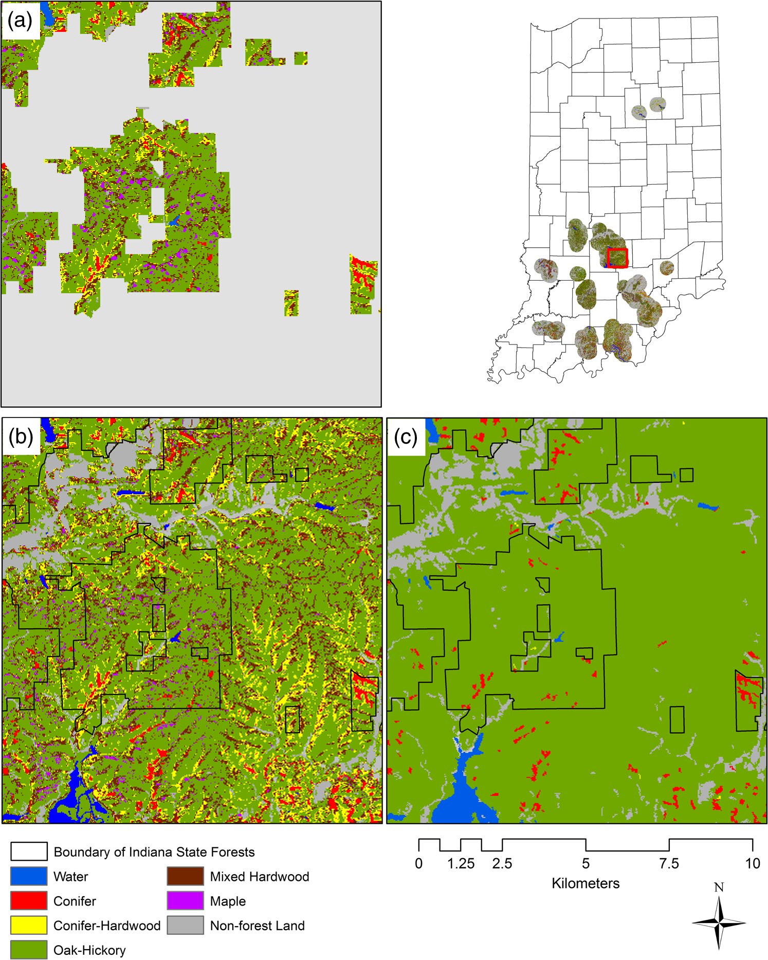

The FFC map resulting from the first stage of the classifications reached an overall accuracy of 74.2% (Table 3). The quantity and allocation disagreements were 0.052 and 0.206. The total disagreement was 0.258.⁴⁶ The oak-hickory forest type had the highest accuracy on the average of user’s and producer’s accuracies, followed by conifer, conifer-hardwood, maple, and mixed hardwood forests. The classification accuracies of conifer-hardwood, maple, and mixed hardwood forests were lower than desirable. The second stage of the classifications increased the overall accuracy to 81.9% (Table 4), better than the 78% overall accuracy of NLCD 2006 level II classification [Fig. 4(c)].⁴⁹ The total disagreement was 0.176 with a quantity disagreement of 0.028 and allocation disagreement of 0.148. Again, the oak-hickory forest type had the highest accuracy; conifer and maple forest types also had satisfactory accuracies. The mixed hardwood forest type had a rather low producer’s accuracy though its user’s accuracy was relatively high. McNemar’s test was applied to compare the results from the first and second stages of the classification. There were 73 plot samples that were used in the second stage of the classification but were not used in the first stage of the classification because they were located in the 8-km surrounding areas of ISF. As McNemar’s test requires the same quantity of samples from these two matrices, these 73 samples were not used in the McNemar’s test, among which, 7 samples were misclassified in the second stage of the classification. The $Z$ value of the McNemar’s test was 2.98, which was $>1.96$. Therefore, the difference of the results from the two classification stages was statistically significant at a 96% confidence level, which means that the result in the second stage of classification was significantly improved.

Table 3

An error matrix of classification for forests within Indiana State Forest following the stage one classification.

Table 4

An error matrix of classification for forests in Indiana State Forest and the 8-km surrounding areas following the stage two classification.

The FFC map shows the dominant compositions of oak-hickory and mixed hardwood forests in forest landscape, comprising 81% of the forested landscape in areas within ISF [Fig. 5(a)]. This result was consistent with forest composition data reported by IDNR (2008),¹⁰ which were obtained from field observations. Maple forest type in the FFC map constitutes 7% of ISF area, equivalent to the sum of 4% for maple and 3% for bottomland hardwoods (IDNR 2008) [Fig. 5(b)]. The combined area of conifer and conifer-hardwood mixed forests in the FFC map was slightly more than the pine forest area reported by IDNR (2008). The proportion of conifer-hardwood forest in the FFC map was reasonable when compared with independent forest inventory and analysis (FIA) data from USDA Forest Service.⁵⁰ The conifer-hardwood forest covered a much larger area in the FFC map than in NLCD 2006 data either inside or outside ISF and is much more detailed than the forest cover classifications in NLCD 2006 [Fig. 5(c)].

Fig. 5

A comparison of forest composition in area among NLCD 2006 (a), five-forest-class map (b), and report by IDNR (2008) (c) for ISF.

5.

Discussion

This study is the first demonstration of the DUC algorithm³⁰ for a real-world classification exercise with an integration of remotely sensed and plot-based forest data. Lang et al.³⁰ designed and tested the DUC algorithm to classify several sample sites into four general land covers, including agriculture, forest, urban, and water. In this study, we applied this algorithm to a much larger site, the ISF with the 8-km surrounding areas. We focused on and split the forests into more detailed forest types, which was more difficult than the general land cover classification due to the similarities. The classification accuracy of such an unsupervised classification approach is determined mainly by imagery quality and sample data. The two-season Landsat TM datasets we used in this study provide richer spectral information than single-season imagery for the classifications of hardwood forests. The CFI plots used in this study were abundant though their distribution among forest types was uneven. All these factors contributed to the development of the FFC map that is reasonably consistent with field survey data. This shows that the integration of image data and forest field data has made the resultant forest cover map more realistic and objective than the use of image data alone.

The overall accuracy of the forest cover map derived at the second stage was unexpectedly greater than that at the first stage. The reason for this phenomenon may be that spectral classes derived from a larger forest area (ISF and the 8-km surrounding areas) have better representations to forest types than those from a smaller forest area (ISF). Because most sample points are located inside ISF, forest cover information within ISF may be more reliable than that outside ISF. The producer’s accuracy of maple forest type in the second stage was lower than that in the first stage; however, the user’s accuracy had significant increases. This means the FFC map created in the first stage overestimated the maple. The FFC of the second stage showed a lower quantity disagreement. It is also reasonable for the additional misclassified maple plots dropping into oak-hickory forest type because maples are shade tolerance species and are usually suppressed under the oak-hickory forests. The same trend of accuracies happened in mixed hardwood forest, where the producer’s accuracy decreased and the user’s accuracy increased. However, there was no confidential evidence to show that mixed hardwood was overestimated in the first stage. FFC in the second stage might have underestimated the mixed hardwood because the total number of mixed hardwood samples in the resultant map was much smaller than that in the reference data. The decrease of the allocation disagreement showed that FFC in the second stage would likely have a better quality.

The classification accuracy is also affected, in theory, by spatial mismatch between pixel coordinates and plot locations. The coordinates of the CFI plots used in this study were measured with handheld global positioning system (GPS) receivers and their errors are normally up to 10 m.⁵¹ The combination of the GPS error and TM image geometric error can be problematic for heterogeneous forest canopies. The coverage of this type of forest inventory data is available for limited forest areas, geographically restricting the applications of the data-assisted unsupervised classifications.

Given the first experiment with the classification method, we suggest that it should be broadly applied with the following considerations:

An important feature of the DUC algorithm is its repeatability, meaning that the classification procedure can be systematically modified by simply changing classification parameters and labeling rules if classification results are not satisfactory, thus the loops in the flow chart of the two-stage unsupervised classification (Fig. 2). Our experience indicates that an automated computer program for recoding can make the classification less labor intensive and reduce human errors in labeling processes despite hundreds of spectral classes. Analysts only need to have fundamental remote sensing training to implement this classification technique.

Forest inventory data, such as FIA, have been used in various ways to improve forest assessment together with remotely sensed imagery.^40,53,54 If researchers can access the exact FIA plot locations, the FIA-DUC approach can be broadly applied at the regional and national scales in the United States. Such a forest mapping procedure will help save time and money due to a reduction in the necessary ground validation.

6.

Conclusions

This study demonstrates the first application of the DUC algorithm in dividing hardwood forests into three forest types in an objective fashion. The overall quality of the resultant forest cover map suggests that the DUC approach with forest inventory data is an effective and efficient method for mapping forest cover in Indiana. However, current ground data do not allow us to classify the hardwood forest into even more detailed levels with satisfactory accuracy. A stepwise classification procedure of species composition overcomes the difficulties caused by the extremely uneven distribution of ground data. The two-stage DUC algorithm successfully extends the mapping area to 8 km away from the plot-based forest data without jeopardizing classification accuracy. This forest mapping technique is suitable for mapping other forest areas where extensive plot data are available.

A forest cover map needs to be noise free if it is to be used for forest management activities in the field. In other words, the minimum mapping unit will likely be greater than pixel size of the remote sensing imagery at a proper scale based on the objective of the map to reduce salt-and-pepper or noise pixels. A forest cover map derived from pixel-based classifications can be filtered to remove noise pixels by using image processing algorithms, such as connected component analysis and morphology fundamentals processing. It is also possible to integrate spectral classes with image segmentation to obtain patch-style spectral classes, based on which labeling procedure is implemented. Such comprehensive experiments need systematic explorations in the future.