Pattern recognition model for aerosol classification with atmospheric backscatter lidars: principles and simulations

Dong Liu; Yongying Yang; Yupeng Zhang; Zhongtao Cheng; Zhifei Wang; Jing Luo; Lin Su; Liming Yang; Yibing Shen; Jian Bai; Kaiwei Wang

doi:10.1117/1.JRS.9.096006

21 September 2015 Pattern recognition model for aerosol classification with atmospheric backscatter lidars: principles and simulations

Dong Liu, Yongying Yang, Yupeng Zhang, Zhongtao Cheng, Zhifei Wang, Jing Luo, Lin Su, Liming Yang, Yibing Shen, Jian Bai, Kaiwei Wang

Author Affiliations +

Journal of Applied Remote Sensing, Vol. 9, Issue 1, 096006 (September 2015). https://doi.org/10.1117/1.JRS.9.096006

Abstract

A pattern recognition model for aerosol classification with atmospheric backscatter lidars is proposed and studied in detail. The theoretical framework and the implementation process of the proposed model are presented. Computer simulations have been carried out to verify the practicability and robustness of this model. The k-fold cross-validation method is employed in the process of classifier designing to choose the proper decision rule, which is mainly based on statistical pattern recognition theory. At the same time, the validity of the model is evaluated. The generalized self-validation is also carried out in the computer simulations to verify the stability of the model. The analysis of the performances in reduced status, especially the instance of application to Cloud-Aerosol Lidar with Orthogonal Polarization, demonstrates the generalization ability and performance of this model.

1. Introduction

Air pollution is becoming more and more serious in China and it is well understood that more should be known before we could control it. Many methods have been proposed for component analysis of haze. Using offline analysis means one can analyze the air samples comprehensively and accurately, but the analyses are time consuming and cannot represent the original characteristics of the aerosols as the chemical components of aerosols are susceptible to be changed. Real-time online means, including mass spectrometry of single particle aerosols and some in situ detection instruments (such as hygroscopic tandem differential mobility analyzers and cavity ring down spectroscopy) may analyze the components of aerosol continuously.¹^,² However, these methods can only work by single-point sampling in a limited area and thus are impractical to employ for analysis over a larger area.

On the contrary, remote sensing methods have very good prospects as they can obtain observation data on a larger scale and can detect the air pollution and distribution of aerosols rapidly without being placed in the detected air.³^,⁴ In particular, lidar is very suitable for remote sensing of atmospheric aerosols because of its high spatial and temporal resolution, and can be developed for vehicular and airborne application.⁵^,⁶ Many observation data have been obtained from the lidar stations and airborne-lidar worldwide, and the optical characteristics of the aerosols can be retrieved from the raw data. Aerosol type classification from atmospheric lidar remote sensing is important to know more about the different effects of aerosols from one type to another type.

In the authors’ previous work, a coarse pattern recognition model was proposed for aerosol identification with atmospheric backscatter lidars.⁷ In this paper, the principle and implementation process of this method is enriched and described in more detail. Computer simulation shows dual-wavelength polarized high-spectral resolution lidar (HSRL) is better than other types of lidars for the classification of aerosols. Moreover, validation and analysis using the data from Cloud-Aerosol Lidar with Orthogonal Polarization (CALIOP) reveal that this model for aerosol classification can be used widely in the analysis of the lidar data.

This paper is constructed as follows. The optical properties of aerosol that could be employed to construct the optical feature vector of the pattern recognition model are briefly reviewed in Sec. 2. Section 3 gives a detailed description of the construction of the pattern recognition model, which is followed by simulation studies in Sec. 4. To validate the proposed model, the application to CALIOP is analyzed in Sec. 5. Section 6 gives the conclusive remarks of this paper.

2. Optical Properties of Aerosol

With elastic backscatter lidar, some optical properties of aerosol can be retrieved, such as backscatter coefficient, depolarization ratio, color ratio, and so on. Some of these optical properties are important for aerosol type classification, and are required input data for the pattern recognition model.

a. Lidar ratio
Backscatter coefficient $β$ and extinction coefficient $α$ can be retrieved from the standard elastic backscatter lidar equation⁸
Eq. (1)
${\begin{cases} P^{∥} (r) = \frac{C^{∥}}{r^{2}} Ψ [β_{m}^{∥} (r) + β_{a}^{∥} (r)] \exp {- 2 \int_{0}^{r} [α_{m} (ξ) + α_{a} (ξ)] d ξ} \\ P^{⊥} (r) = \frac{C^{⊥}}{r^{2}} Ψ [β_{m}^{⊥} (r) + β_{a}^{⊥} (r)] \exp {- 2 \int_{0}^{r} [α_{m} (ξ) + α_{a} (ξ)] d ξ} \end{cases},$
where $P^{∥}$ and $P^{⊥}$ represent the backscatter signals from parallel and perpendicular channels, respectively; $C^{∥}$ and $C^{⊥}$ represent the system constants for the parallel and perpendicular channels, respectively; $r$ is the range of the scatter volume from the lidar, $Ψ$ is the transmitter-receiver geometric overlap function. The subscripts $m$ and $a$ represent the molecule and aerosols, respectively. Standard elastic backscatter lidars often need to assume the lidar ratio (aerosol extinction-to-backscatter ratio) in advance as there are three unknowns ( $β_{a}^{∥}$ , $β_{a}^{⊥}$ , $α_{a}$ ) in two lidar equations,⁹ that is,
Eq. (2)
$S_{a} = α_{a} / β_{a} .$
b. Optical depth
The aerosol optical depth (AOD) refers to the integral of atmospheric extinction coefficient in vertical direction, which can be used to describe the attenuation effect to light of the atmospheric aerosol. That is,
Eq. (3)
$τ = τ_{a} + τ_{m} = \int_{0}^{r} [α_{a} (ξ) + α_{m} (ξ)] d ξ .$
The extinction angstrom exponent is often used to parameterize the wavelength behavior of AOD. The relationship between the AOD and the wavelength is described as follows:¹⁰
Eq. (4)
$τ_{a} (λ) = B λ^{- A},$
such that
Eq. (5)
$A = \frac{- \ln [τ_{a} (λ_{1}) / τ_{a} (λ_{2})]}{\ln (λ_{1} / λ_{2})},$
where $B$ represents the turbidity coefficient of aerosols, $λ_{1}$ and $λ_{2}$ represent two reference wavelengths, $A$ represents the angstrom wavelength exponent, which is an important optical parameter to describe the size of aerosol particles. The greater its value is, the smaller the particle is and vice versa.
c. Color ratio
The backscatter-related angstrom exponent is often used to characterize aerosols, and can be expressed as
Eq. (6)
$a_{β} = - \ln (β_{a}^{532} / β_{a}^{1064}) / \ln (532 nm / 1064 nm),$
where $β_{a}^{i}$ represents the aerosol backscatter coefficient at wavelength $i$ , $C_{a} = β_{a}^{532} / β_{a}^{1064}$ represents the backscatter color ratio, which is independent of the particle concentration.¹¹ The Angstrom exponent $α_{β}$ is related to the size of aerosol particles and is typically below 0.5 for larger dust particles, whereas it is bigger than 1 for anthropogenic particles.¹²
d. Depolarization ratio
There are also two important parameters derived from the backscatter coefficient. One of them is the particle linear depolarization ratio
Eq. (7)
$δ_{a} = β_{a}^{⊥} / β_{a}^{∥},$
and the other is the spectral depolarization ratio
Eq. (8)
$R_{a} = δ_{a}^{1064} / δ_{a}^{532} .$

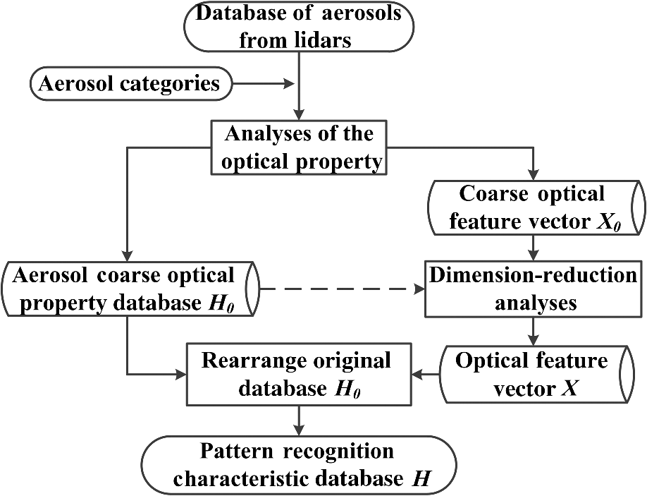
The atmospheric aerosols optical parameters (such as the depolarization ratio, lidar ratio and so on) are closely related to the physical properties of the particles. These optical parameters of different kinds of particles are not exactly the same at a single wavelength and each parameter also varies with the wavelength. Taking the depolarization ratio as an example, researchers found that pure dust has typically larger 532-nm depolarization ratio (up to 30% to 35%)¹³ and that of a mixture of dust and spherical particles is about 8% to 10%.¹⁴ In terms of aerosol lidar ratio, it can vary widely depending on aerosol size distribution and refractive index, and the aerosol lidar ratio is highly variable (20 to 100 sr). The mean values of lidar ratio for urban aerosols and biomass burning are much higher than those for aerosols from maritime or dust aerosols at visible wavelength (550 nm of AERONET or 532 nm of Raman lidar), which make them separable.¹⁵^–¹⁷ Therefore, it is not hard to understand that these optical characteristic parameters (such as depolarization ratio, lidar ratio and so on) play an indispensable role in aerosol classification.

Moreover, it is necessary to point out how can obtain the aforementioned optical parameters. Standard elastic backscatter lidars need to assume lidar ratio in advance, then a single-wavelength polarized Mie lidar can retrieve the depolarization ratio $δ_{a}$ and a dual-wavelength Mie lidar with polarized sensitivity only at 532 nm, which is widely adopted in the AD-net and satellite-based lidar (CALIOP) at present,¹⁸^,¹⁹ can retrieve the depolarization ratio $δ_{a}$ along with the color ratio $C_{a}$ . It should be noted that even with elastic backscatter lidar, the optical properties of aerosol can be retrieved with a certain degree of accuracy. However, HSRL, which is obtained by adding spectral filters to standard Mie lidar, can solve the optical parameters of the aerosol particles (extinction coefficient $α_{a}$ and backscatter coefficient $β_{a}$ ) accurately without a priori assumptions of lidar ratio because it can obtain an extra lidar equation by separating the Mie scattering of the aerosols and the Rayleigh scattering of the atmospheric molecules.²⁰^–²² Thus, a single-wavelength polarized HSRL can retrieve the depolarization ratio $δ_{a}$ and lidar ratio $S_{a}$ , and a dual-wavelength polarized HSRL can retrieve the depolarization ratio $δ_{a}$ , spectral depolarization ratio $R_{a}$ , backscatter color ratio $C_{a}$ , and lidar ratio $S_{a}$ accurately as it can work on two wavelengths.

3. Model for Aerosol Classification with Atmospheric Backscatter Lidars

A pattern recognition model for aerosol classification with atmospheric backscatter lidars can be built up based on measured optical properties of aerosols from lidars, as shown in Fig. 1. In general, the main process of this model can be described as follows. First, one must design the pattern recognition classifier for aerosol classification with atmospheric backscatter lidars. Obtaining the decision function for pattern recognition is the key for this stage. To this end, the pattern recognition characteristic database is divided into two parts, one of which is used as the “database” and the other is used as the “training data,” so the proper decision function and rule can be chosen according to the identification results. Then, input the samples to be identified into the designed classifier, which consists of the pattern recognition characteristic database and the decision rule. Finally, the classification results can be made according to the decision rule.

Fig. 1

Principle diagram of aerosol classification with atmospheric remote sensing lidars based on pattern recognition.

3.1.

Characteristics Sample Database for Aerosol Identification

From the principle block diagram shown in Fig. 1, it is not hard to find that the establishment of the pattern recognition characteristic database is an important step to implement the aerosol identification. Figure 2 shows the process of establishing the pattern recognition characteristic database. First, one can obtain the coarse optical feature vector $X_{0}$ and aerosol coarse optical property database $H_{0}$ by analyzing the collected database of aerosols from lidars according to the existing categories of aerosols. Then, considering the efficiency and complexity of the model in the practical applications, we should reduce the dimension of $X_{0}$ by dimension-reduction analysis, and we can gain the final optical feature vector $X$ used in the model. Finally, the pattern recognition characteristics database $H$ would be obtained by dealing with the aerosol coarse optical property database $H_{0}$ according to the final optical feature vector $X$ .

Fig. 2

The establishment of the pattern recognition characteristic database.

Dimension-reduction analysis can be mainly achieved through feature extraction and feature selection, which is an essential issue in the pattern recognition, and has been proven in both theory and practice effective in enhancing learning efficiency, increasing predictive accuracy, and reducing complexity of learned results.²³ Feature extraction requires processing of data fusion and creating new features based on transformations or combinations of the original feature set.²⁴ Feature selection aims to choose an optimal feature subset that contains just the relevant and nonredundant features for the classifier from the input feature set. Many methods have been developed for feature selection, which can be characterized as “embedded,” “filter,” or “wrapper” approaches.²⁵ As it is not the focus of this paper, readers can learn more about it from related studies.²³^–²⁷ It is worth noting that as many studies have been done and there is clear meaning for the lidar retrieval results, feature selection should be employed if only lidar data were considered. If multisource data have been used for aerosol classification, feature extraction should be considered first, as features can be extracted from the raw data after a series of translation. Thus, a correlation-based feature selection method was adopted to aid the dimension-reduction analysis. The correlation between any feature and the class (C-correlation) as well as the correlation between any pair of features (F-correlation) should be considered. Then, relevant and nonredundant feature subset can be gained by selecting the features that have high C-correlation as well as low F-correlation with each other.²³

In conclusion, the pattern recognition characteristic database $H$ has been simplified and the superfluous optical properties have been eliminated when compared with the aerosol coarse optical property database. Thus, a more accurate and efficient pattern recognition can be realized.

3.2.

Decision Rules

Once the pattern recognition characteristic database for aerosol classification has been established, the classifier can be designed using a number of possible approaches, such as template matching, statistical classification, syntactic or structural matching, neural networks, and so on. Statistical pattern recognition is a very active area of study and research, which has been used successfully to design a number of commercial recognition systems. In the statistical decision theoretic approach, the decision boundaries are determined by the probability distributions of the samples belonging to each class or estimated directly by the data without calculating the probability distributions.²⁸ However, in some sense, most of the approaches in statistical pattern recognition are attempting to implement the Bayes decision rule as the Bayes discriminant method based on the Bayes theory has the minimum error rate compared with other classification methods theoretically.²⁹

If the feature vector of the sample to be identified is $x$ , the probability of the sample belonging to aerosol category $ω_{i}$ in all $n$ -type aerosols can be described as

Eq. (9)

P (ω_{i} | x) = \frac{P (x | ω_{i}) P (ω_{i})}{\sum_{j = 1}^{n} P (x | ω_{j}) P (ω_{j})}, i = 1,2, 3, \dots n,

where

P (ω_{i})

represents the prior probability, which can be assigned as equal for all types of aerosols or calculated statistically or even determined experientially, and

P (x | ω_{i})

represents the probability distribution of the aerosol category

ω_{i}

. Burton et al.³⁰ and Cattrall et al.¹⁶ pointed out that various kinds of aerosol characteristic sample database can be considered to obey the multidimensional Gaussian distribution as

Eq. (10)

P (x | ω_{i}) = 1 / [{(2 π)}^{d / 2} {| Σ_{i} |}^{1 / 2}] \exp {- \frac{1}{2} {(x - μ_{i})}^{T} Σ_{i}^{- 1} (x - μ_{i})},

where

x = {(x_{1}, x_{2}, \dots x_{d})}^{T}

represents the

d

-dimension feature vector,

μ_{i} = {(μ_{1}, μ_{2}, \dots μ_{d})}^{T}

represents the

d

-dimension mean vector of class

ω_{i}

,

Σ_{i}

represents the

d \times d

-dimension covariance matrix of class

ω_{i}

, which is defined as

Σ_{i} = E {(x - μ_{i}) {(x - μ_{i})}^{T}}

, and

Σ_{i}^{- 1}

represents the inverse matrix of

Σ_{i}

.

As can be seen, if one estimates the parameters of the multidimensional Gaussian distribution according to the experimental data, $P (x | ω_{i})$ can be gained by Eq. (10). Then, $P (ω_{i} | x)$ , the relative probability of the aerosol sample belonging to class $ω_{i}$ , can be obtained subsequently. Decision rules can be set in two ways: one is to select the maximum relative probability to be the result of aerosol classification. That is, if $P (ω_{i} | x) = \max_{j = 1,2, \dots, n} P (ω_{j} | x)$ , then $x \in ω_{i}$ . However, the crosstalk between two different types of aerosols may be very strong in some cases. The other is to set a threshold if a rejection decision is allowed. If the relative probability of the aerosol sample belonging to class $ω_{i}$ is larger than the threshold, the aerosol sample can be considered as this kind of aerosol.

Based on the preceding analysis, a refined pattern recognition characteristic database can be obtained from the atmospheric backscatter lidar observation according to the method introduced in the Sec. 3.1. Then, it is divided into two parts: one is treated as the database and the other is used as a set of training data, as shown in Fig. 1. A satisfying self-validation would be obtained by choosing a proper decision rule, and this decision rule combining with the pattern recognition characteristic database forms the classifier. Therefore, the aerosol classification can be made. As there are wrongly classified samples, the confident level of the classification results can be evaluated by

Eq. (11)

C (ω_{i}) = \frac{P (ω_{i}, ω_{i}) P (ω_{i})}{\sum_{j = 1}^{n} P (ω_{i}, ω_{j}) P (ω_{j})}, i = 1,2, 3, \dots n,

where

C (ω_{i})

represents the classification confident level of aerosol category

ω_{i}

and

P (ω_{i}, ω_{j})

represents the relative probability of samples from class

ω_{j}

classifying into class

ω_{i}

. It is worth noting that though classification accuracy is the primary evaluation criterion for the classification results, the confidence levels should be taken into account as well.

4. Analysis of Computer Simulation

Computer simulation for the proposed pattern recognition model of aerosol identification has been carried out and the results will be shown in this section.

4.1.

Establishment of Model

4.1.1.

Aerosol categories

Aerosols can be categorized in different ways and different databases can be built up correspondingly. The aerosol categories should be chosen according to the regional real situation, and the number of aerosol categories should neither too few nor too many. Here, in this study, aerosols are divided into eight categories: ice particles, pure dust, dust mix, maritime, marine pollution, urban aerosol, biomass burning, and fresh smoke, following Burton et al.³⁰

4.1.2.

Selection of aerosol feature vector

As we are classifying the aerosols, it is interesting to find that some optical characteristics of aerosols, such as depolarization ratio, spectrum depolarization ratio, backscatter color ratio, and lidar ratio, do not change over the concentration of aerosols.¹¹^,¹⁶^,³⁰ One or two of the four characteristics are usually not quite similar among different kinds of aerosols. Therefore, it has a great significance in the classification of aerosols.

As for quantitative analysis, a large number of measurements of known aerosol models were carried out to gain the optical characteristics of various kinds of aerosols. Therefore, the aerosol database can be built up with atmospheric backscatter lidars. After dimension-reduction analysis to the aerosol coarse optical property database according to the previous analysis, we found that the four optical characteristic parameters particle linear depolarization ratio (at 532 nm), lidar ratio (at 532 nm), backscatter color ratio and spectrum depolarization ratio have high C-correlation and the correlation between any pair of these four features are quite low. Thus, feature vector for aerosol classification can be selected as follows:

Eq. (12)

x = {(δ_{a}^{532}, S_{a}^{532}, C_{a}, R_{a})}^{T} .

Then, the four-dimension feature vector space of aerosol particles can be constructed. Thus, we can focus on these four characteristics specifically in the process of establishing the sample database. The database can be stored for later use.

4.1.3.

Characteristics sample database for aerosol identification

The characteristics sample database for aerosol identification used in the computer simulation is constructed from the experimental data of Burton et al.,³⁰ which are obtained in the field task over North America. There are 10,000 samples of ice particles, 3000 samples of pure dusts, 75,000 samples of dust mix, 13,000 maritime samples, 11,000 samples of marine pollution, 85,000 samples of urban aerosols, 22,000 samples of biomass burning, and 39,000 samples of fresh smoke in the database. The projection distribution of the four-dimension feature space for aerosol classification is shown in Fig. 3,⁷ where (a) represents the projection in 532-nm depolarization—532-nm lidar ratio space, (b) represents the projection in 532-nm depolarization—backscatter color ratio space, (c) represents the projection in 532-nm depolarization—depolarization spectral ratio space, and (d)–(f) represent the projection in 532-nm lidar ratio—backscatter color ratio space, the projection in 532-nm lidar ratio—depolarization spectral ratio space, the projection in backscatter color ratio—depolarization spectral ratio space, respectively.

Fig. 3

Aerosol database used in computer simulation: (a) projection in 532-nm depolarization—532-nm lidar ratio space, (b) projection in 532-nm depolarization—backscatter color ratio space, (c) projection in 532-nm depolarization—depolarization spectral ratio space, (d) projection in 532-nm lidar ratio—backscatter color ratio space, (e) projection in 532-nm lidar ratio—depolarization spectral ratio space, and (f) projection in backscatter color ratio—depolarization spectral ratio space.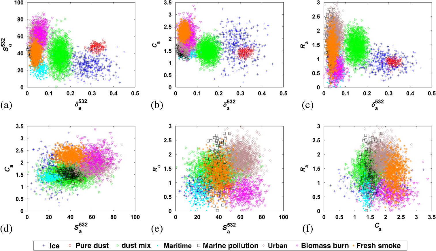

4.2.

Self-Validation Accuracy

The aerosol classification system is operated in two steps: training (learning) and classification (testing). Two self-validations were carried out in the computer simulations to test the validity and stability of the pattern recognition model for aerosol identification with atmospheric backscatter lidars in these two processes, respectively.

In the process of classifier training, the strict self-validation was carried out to determine the decision rule. As shown in Fig. 1, the characteristics sample database was divided into two parts: one was treated as the pattern recognition database and the other was used as train data. We adopt the $k$ -fold cross-validation method³¹ considering that the number of pure dust sample points is relatively few. First, the characteristics sample database was divided into 50 parts randomly; second, a decision function was selected; third, we pick one part as the training data and the remained 49 parts as the pattern recognition database to train the classifier. This is repeated for 50 times with only picking different parts as the training data each time. In this way, the accuracy of the classifier with a certain decision rule can be calculated by recording and adding the results of 50 cycles.

At first, we adopt the first decision rule to design the classifier, that is, we calculate the relative probability of the aerosols belonging to any kind of categories and label the aerosol sample belonging to this category if the probability is maximal. The detailed analysis results of strict self-validation are shown in Fig. 4(a). The vertical axis in the figure represents the types of aerosol to be tested in the self-validation, and the horizontal axis represents the categories of aerosol in which the samples are classified into. The light and dark colors represent the corresponding probabilities. For example, look at the row with a vertical axis of “ice,” the first dark blue square with a horizontal axis of “ice” represents samples of ice is still classified as ice, and how dark of the square represents the corresponding probability in proportion to the total ice sample points according to the color bar in the bottom of the figure. The second light blue square with a horizontal axis of “pure dust” represents the samples of ice are classified as pure dust mistakenly, and the rest may be deduced by analogy. Some of the self-validation accuracies are marked correspondingly in the figure, but the corresponding probabilities less than 1% are not marked in the figure.

Fig. 4

Details of the strict self-validation results: (a) the accuracies of strict self-validation without decision threshold and (b) the accuracies of strict self-validation with decision threshold.

From the results of self-validation, we can find that the reidentification of urban aerosol is the most difficult and only about 89% of the sample points can be correctly distinguished. The main reason is that the overlapping area of urban with other kinds of aerosol categories is larger than the others, especially in the 532-nm depolarization—backscatter color ratio space [see Fig. 3(b)] and 532-nm lidar ratio—backscatter color ratio space [see Fig. 3(c)], where urban almost cannot be separated from other kinds of aerosols. Meanwhile, the accuracies of maritime pollution aerosol and fresh smoke are relatively low, too. This is mainly because the feature vectors of these two types of categories overlap with urban aerosol as the crosstalk among them is quite serious. The reidentification accuracies of other five types of aerosols, such as ice and dust mixing, reach 94% or even more. The pure dust is reidentified almost without error.

Obviously, the crosstalk between different types of aerosols will lower the confidence of the classification results. Maybe adopting a rejection decision with a threshold as described in Sec. 3.2 would make the classification results more confident. After a process of analysis, a threshold of 55% was adopted in the classifier. That is, we use the $k$ -fold cross-validation method introduced earlier and calculate the relative probability of the aerosol sample belonging to any kind of aerosol. Then, we can consider the aerosol sample belonging to this kind of aerosol if the probability is over 55%. The detailed analysis results of self-validation with a proper threshold are shown in Fig. 4(b).

From the self-validation result shown in Fig. 4(b), one can see that the reidentification accuracies of eight types of aerosols are lower compared to the self-validation results without a threshold, but the crosstalk is reduced in the meantime. In the further analysis, it is noticed that the effects of setting a threshold to the validation accuracies of ice, pure dust, dust mix, and maritime samples are quite small, which means that the classification results of these four types of aerosols are relatively confident. Thus, it is necessary to set a threshold if a confident result is required. A best threshold should be decided by the data of repeated experiments according to practical needs.

After the classifier is designed, the generalized self-validation was carried out in the classification mode. The testing data are simulated samples, which have the same distribution but different values with the pattern recognition characteristic database. We still set the threshold at 55% and the generalized self-validation accuracies of eight types of aerosols are shown in Fig. 5(a). We carried out simulations four times and an average is calculated and marked out correspondingly in the figure. It can be seen that the results of strict self-validation and generalized self-validation are very close. Therefore, we believe that the results of self-validation are close to a stable state. Thus, a change of the value of sample points would not affect the reidentification results a lot as long as the distribution of the used database is the same. The crosstalk between each type of aerosol in the generalized self-validation is similar to that in the strict self-validation; thus, we will not discuss the crosstalk issue in the generalized self-validation further.

Fig. 5

Results of the generalized self-validation and sensitivity analysis: (a) the generalized self-validation accuracies of eight types of aerosols and (b) classification results of sensitivity analysis with different uncertainties.

In addition, we carried out a sensitivity analysis by perturbing each sample point in the pattern recognition characteristic database 1000 times within different measurement uncertainties as testing data, and the classification accuracies of eight categories of aerosols are shown in Fig. 5(b). From the results, we can see that the effects of measurement uncertainties on classification accuracies of ice, dust mix, maritime, and biomass burn are relatively low. Nevertheless, the classification accuracies of pure dust and fresh smoke are affected relatively seriously by the measurement uncertainties. In the whole, the effects of measurement uncertainties of less than 15% are quite acceptable.

However, it should be pointed out that in order to obtain these four characteristic parameters of aerosol at the same time, dual-wavelength polarized HSRL would be the best choice. Yet, dual-wavelength polarized HSRL has not been widely accepted and used because of the restriction of research depth and technology. The single-wavelength HSRL (at 532 nm) and other atmospheric remote sensing equipment (such as single-wavelength polarization Mie scattering lidar) are usually used together to obtain all of these optical characteristic parameters at present.

4.3.

Behavior in a Reduced Dimension Status

As most lidars used currently are not dual-wavelength polarized HSRLs and a joint measurement of different equipment is also hard to carry out, it is difficult to obtain all the four optical characteristic (depolarization ratio $δ_{a}$ , spectral depolarization ratio $R_{a}$ , backscatter color ratio $C_{a}$ , and lidar ratio $S_{a}$ ) at the same time. As mentioned earlier, a dual-wavelength Mie lidar with polarized sensitivity at 532 nm can only retrieve the depolarization ratio $δ_{a}$ and the color ratio $C_{a}$ , a single-wavelength polarized HSRL can only retrieve depolarization ratio $δ_{a}$ and lidar ratio $S_{a}$ , and a single-wavelength polarized Mie lidar can only get depolarization ratio $δ_{a}$ . These limitations make it very difficulty to classify aerosol with atmospheric backscatter lidars. Although the pattern recognition model for aerosol classification with atmospheric backscatter lidars proposed in this paper can be applied to both dual-wavelength polarized HSRL and nondouble-wavelength polarized HSRL, the accuracy would have some differences compared with the results of dual-wavelength polarized HSRL. The results of self-validation for nondouble-wavelength polarized HSRL (such as dual-wavelength Mie lidar with polarized sensitivity at 532-nm, single-wavelength polarized HSRL, single-wavelength polarized Mie lidar, and so on) without a decision threshold are shown Fig. 6.

Fig. 6

Details of the self-validation analysis for nondual-wavelength polarized high-spectral resolution lidar (HSRL) without decision threshold: (a) the self-validation accuracies analysis for double-wavelength Mie scattering lidar (polarized at 532-channel), (b) the self-validation accuracies analysis for single-wavelength polarized HSRL lidar, and (c) the self-validation accuracies analysis for single-wavelength polarized Mie scattering lidar.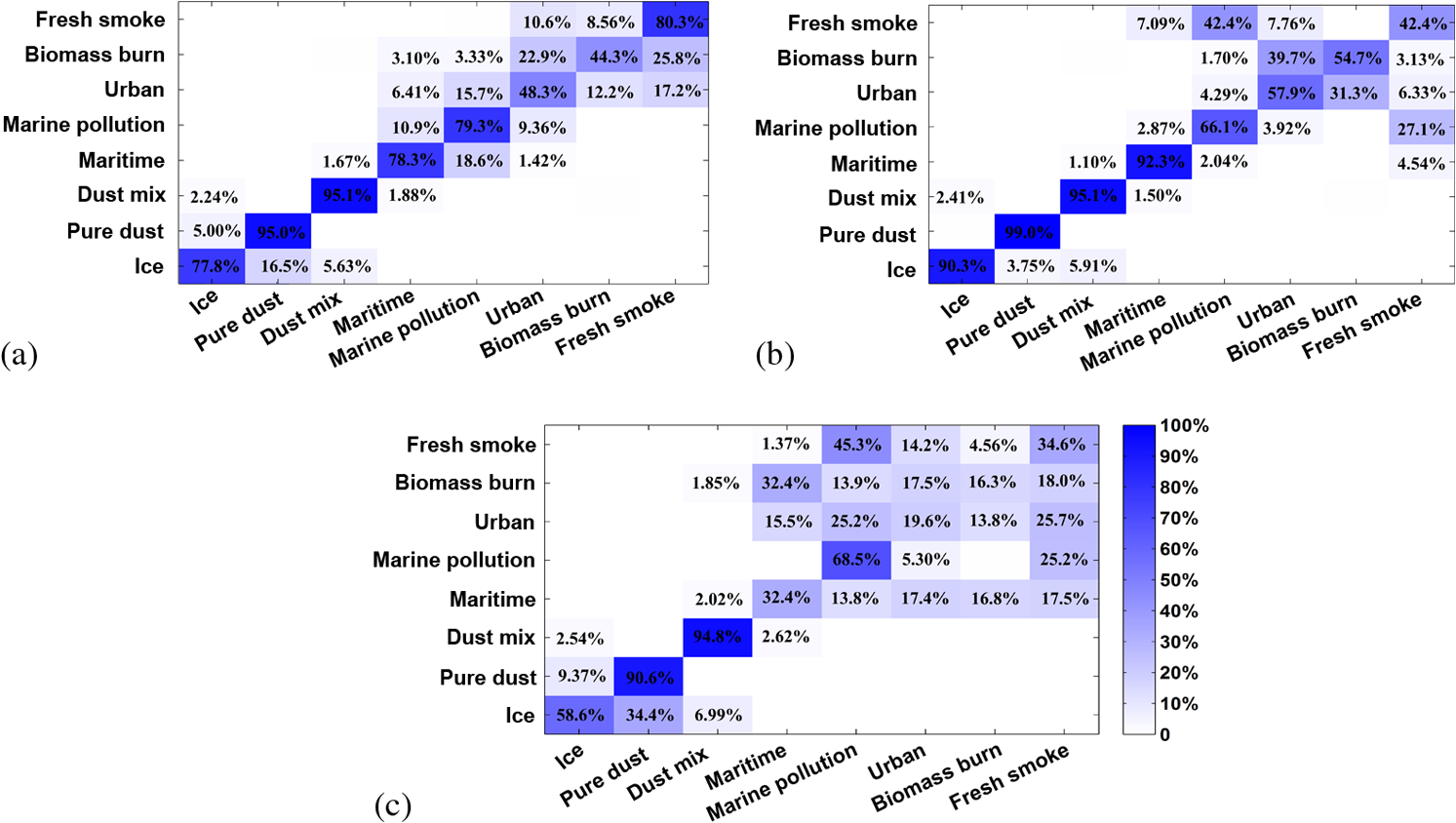

Compared to the self-validation of the dual-wavelength polarized HSRL shown in Fig. 4(a), the reidentification accuracies in a reduced dimension status is lower and the crosstalk becomes worse. Therefore, we decided to adopt a rejection decision by setting a threshold. A threshold of 50% is set by balancing the self-validation accuracies and crosstalk between each type of aerosols. The detailed results of self-validation are shown in Fig. 7.

Fig. 7

The details of self-validation analysis for nondouble-wavelength polarized HSRL with decision threshold: (a) the self-validation accuracies analysis for dual-wavelength Mie scattering lidar (polarized at 532-channel), (b) the self-validation accuracies analysis for single-wavelength polarized HSRL lidar, and (c) the self-validation accuracies analysis for single-wavelength polarized Mie scattering lidar.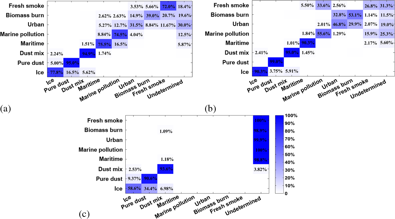

According to the self-validation results, although a single-wavelength polarized HSRL can only obtain depolarization ratio $δ_{a}$ and lidar ratio $S_{a}$ , the distributions of various types of aerosols are relatively independent in the two-dimensional space consisting of depolarization ratio and lidar ratio. Thus, the identification accuracies of various aerosols are still quite large: the reidentification accuracies of ice, pure dust, dust mix, and maritime are all over 90% and the reidentification accuracy of pure dust is up to 99%. However, the reidentification accuracies of other four types of aerosols are quite low and the crosstalk between marine pollution and fresh smoke as well as urban aerosol and biomass burn is quite serious. It seems hard to distinguish urban aerosol from biomass burn only using the data from a single-wavelength polarized HSRL, because these two almost overlap in the 532-nm depolarization—532-nm lidar ratio space, as shown in Fig. 3. The marine pollution and fresh smoke are hard to be distinguished as their overlapping area in the four-optical feature space is quite large, too.

Compared with single-wavelength polarized HSRL, dual-wavelength polarized Mie lidar has a weaker ability to recognize the components of various types of aerosols. It can only distinguish pure dust and dust mix better. However, the crosstalk between pure dust and ice particles is quite serious, up to 16.5%, as the overlap of pure dust and ice particles is a little large in the 532-nm depolarization—color ratio space as shown in Fig. 3. Although the self-validation accuracies of maritime, marine pollution, and fresh smoke are all over 70%, the crosstalk between them and other categories is very serious, which leads to the confidence of the identification results being very low. However, the combination of maritime and marine pollution has relatively little crosstalk compared with the others. Therefore, if we classify aerosols into five categories according to the data from dual-wavelength Mie lidar (polarized at 532-nm channel), the results are quite acceptable.

As for single-wavelength polarized Mie lidar, its ability to classify the aerosols is even weaker. It can only reidentify pure dust and dust mix, and the crosstalk between ice particles and pure dust is even more serious than dual-wavelength polarized Mie lidar. It cannot distinguish the remaining types of aerosols from each other very well just using the data from single-wavelength polarized lidar, so we would consider the remaining of aerosol types (maritime, marine pollution, urban, biomass burn, and fresh smoke) as one category. When setting a threshold of 50%, the classification results are also acceptable.

4.4.

Discussions

According to the results of computer simulation, we can conclude that the self-validation accuracies of dual-wavelength polarized HSRL are relatively high and the crosstalk is quite low. The classification accuracies stay relatively stable when the measurement uncertainties are less than 15%, so the stability of the model has been demonstrated from the generalized self-validation and sensitivity analysis. The analysis of the behavior in the reduced dimension status demonstrates the generalization ability of this model, which means that it can be applied to different polarization lidar configurations. As the crosstalk between marine pollution and fresh smoke as well as that between urban aerosol and biomass burning are quite serious, aerosols can be divided into six categories quite credibly by single-wavelength polarized HSRL. Similarly, a dual-wavelength Mie lidar with polarized sensitivity at 532-nm channel can classify aerosols into five categories at an acceptable confidence level. The ability to classify the aerosols of a single-wavelength polarized lidar is quite weak, but it can distinguish ice particles, pure dust, and dust mix from other aerosols using the method proposed in this paper. It should be noted that the database used is not based on a real dual-wavelength polarized HSRL. In fact, the HSRL used by Burton et al.³⁰ in the field task adopts HSRL technology only at the 532-nm channel and the 1064-nm channel is just a standard polarized Mie lidar that needs a prior assumption of the lidar ratio before retrieving.³² If data from a real dual-wavelength polarized HSRL can be obtained, the self-validation accuracy would be higher and the crosstalk would be suppressed as well.

It should also be mentioned that the aerosols database used in the computer simulation is obtained by simulation through combining the data sets that were acquired from the 18 field missions conducted by NASA LaRC over North America and the previous research of Burton et al.³⁰ Although the database has certain representativeness, it may show some difference with the concrete situation in other countries. Also, the classification of aerosols in different situations may differ, e.g., the space-based lidar, CALIOP, adopts a classification of six categories, which is quite different from the classification categories used by Burton et al.³⁰ Therefore, the validation of the model’s universality is carried out using the data from CALIOP in Sec. 5.

5. Analysis of the Application to Cloud-Aerosol Lidar with Orthogonal Polarization

CALIOP was launched on April 2006 aboard the Cloud-Aerosol Lidar and Infrared Pathfinder Satellite Observation (CALIPSO) satellite, which is a joint mission between NASA and the French space agency (CNES). CALIOP is a system of dual-wavelength Mie lidar with polarization sensitivity (532-nm channel) and its products can be employed in various applications such as atmosphere studied and earth observation.³² The retrieval algorithm of CALIOP is similar to the common elastic lidar as a priori assumptions are needed. The aerosol layers are assigned to one of six aerosol types (desert dust, biomass burning, clean continental, polluted continental, marine, and polluted dust), each having a characteristic lidar ratio that is mainly based on the cluster-analysis of the AERONET data set.³³^,³⁴ Therefore, CALIOP can provide vertical structure and properties of thin clouds and aerosols over the global scale and the data are available on the NASA website.³⁵ In this study, the layer-integrated particulate depolarization ratio, layer-integrated particulate color ratio, layer-integrated attenuated backscatter coefficient (532 nm), and feature classification flags in the level 2 version 3-layer products, namely the 5-km aerosol layer products, were used to verify the aerosol classification model proposed. The data used are limited to the latitude-longitude grid of (3°N∼54°N, 73°E∼136°E) covering the geographical range of China and surrounding areas over the year 2014.

5.1.

Data Quality Screening Strategy

As an estimated lidar ratio was used in the retrieval algorithm of CALIOP, an untrustworthy retrieval result may be gained. In order to include only well-defined aerosol layers, a quality filter was used in the data processing.³⁶ The cloud-aerosol-discrimination (CAD) score was adopted to assess the uncertainty of cloud aerosol discrimination algorithm. The standard CAD score ranges from $- 100$ (most confident to be aerosols) to 100 (most confident to be clouds), but layers with CAD score between $- 20$ and 20 are usually the results of erroneous layer detection contaminated by noise. Therefore, a CAD score filter was set to determine aerosol layers with CAD score between $- 100$ and $- 20$ . In the meanwhile, bit 13 of feature classification flags was limited to 1, which means the subtype of classification was with confidence.

As the lidar ratio is estimated with assumptions, the initial lidar ratio would be adjusted in the retrieval processing, which usually occurs for complex features and induces instabilities in the algorithm and larger uncertainties in the retrieved extinction. Therefore, a quality filter was used to determine aerosol layers having extinction QC flag values of 0 or 1.

The third screening filter excludes samples where aerosol layer-integrated particulate depolarization ratio uncertainty or layer-integrated particulate color ratio uncertainty is 99.99. Uncertainty of 99.99 is a flag value assigned by the extinction retrieval algorithm when the error estimates can become unstable, and the uncertainty calculation value can grow excessively large. The data quality screening filters are shown in Table 1 in detail.

Table 1

The data quality screening strategy of Cloud-Aerosol Lidar with Orthogonal Polarization.

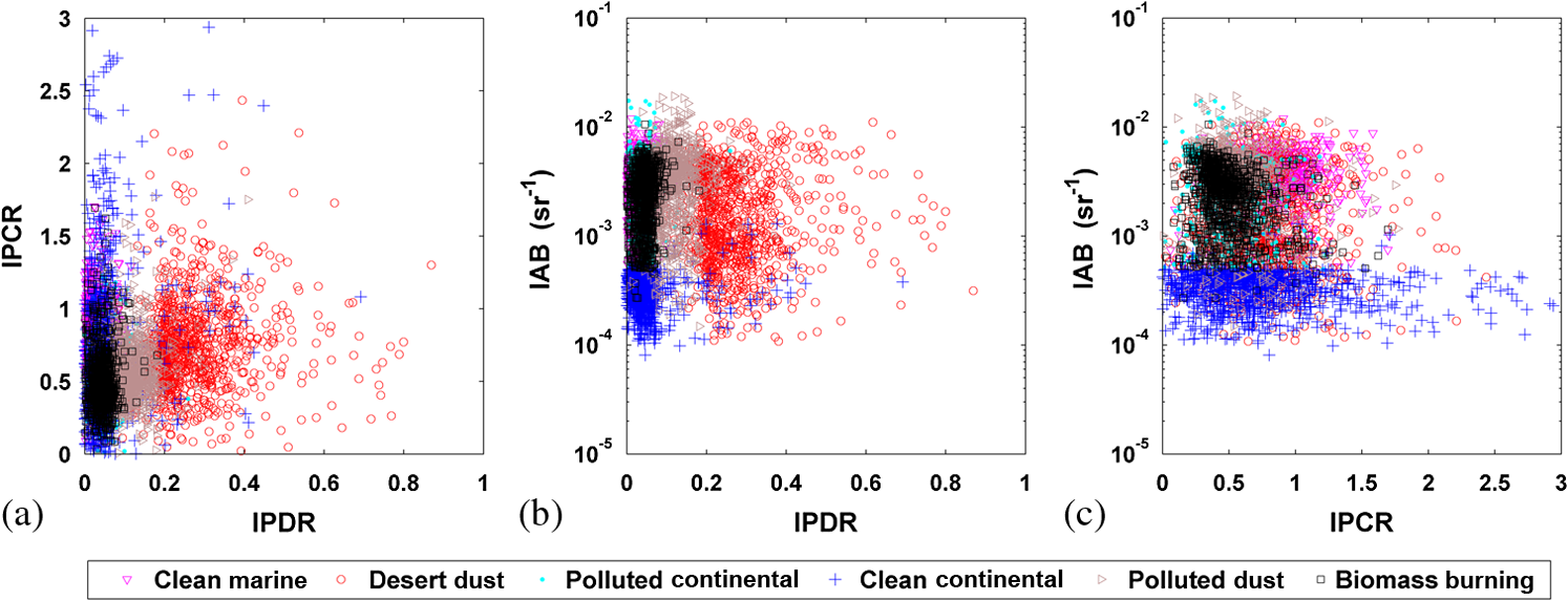
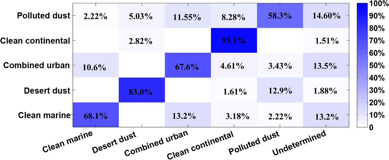
Parameters	Cloud-aerosol-discrimination score	Extinction QC (532 and 1064 channel)	Layer-integrated particulate depolarization ratio uncertainty	Layer-integrated particulate color ratio uncertainty
Filter	$[- 100, - 20)$	0 or 1	Exclude 99.99	Exclude 99.99

5.2.

Selection of Aerosol Feature Vector

Similar to the computer simulation in Sec. 4, the particulate color ratio and depolarization ratio were selected in the feature subset as they are relevant to the classification. Considering that the SNR of satellite-based lidar is relatively low, the integrated particulate depolarization ratio (IPDR)

Eq. (13)

δ_{p, layer} = \sum_{k = top}^{base} β_{⊥, p} (z_{k}) / \sum_{k = top}^{base} β_{∥, p} (z_{k}),

and integrated particulate color ratio (IPCR)

Eq. (14)

χ_{p, layer} = \sum_{k = top}^{base} β_{p, 1064} (z_{k}) / \sum_{k = top}^{base} β_{p, 532} (z_{k}),

are used for aerosol classification instead.

According to the retrieval algorithm, we can see that the integrated attenuated backscatter at 532 nm ( $γ_{532}^{'}$ or IAB) is helpful for aerosol classification. $γ_{532}^{'}$ has a high correlation to classification and low correlation to IPDR or IPCR as well, so $γ_{532}^{'}$ is selected into the feature subset

Eq. (15)

γ_{532}^{'} = \int_{top}^{base} β (z) T (z) d z,

where

β

is the total (molecular + aerosol) backscatter coefficient and

T

is the atmospheric transmittance due to both the molecules and aerosols.

Thus, the feature vector for aerosol classification can be selected as follows:

Eq. (16)

x = {(δ_{p, layer}, χ_{p . layer}, γ_{532}^{'})}^{T} .

Then, the 3-D feature vector space can be gained by analyzing the CALIOP data for year 2014. There are about 130,000 samples of clean marine, 85,000 samples of desert dust, 35,000 samples of polluted continental, 6700 samples of clean continental, 146,000 samples of polluted dust, and 53,000 samples of biomass burning. The projection distribution of the 3-D feature space for aerosol classification is shown in Fig. 8, where (a) represents the projection in IPDR—IPCR space, (b) represents the projection in IPDR—IAB space, and (c) represents the projection in IPCR—IAB space.

Fig. 8

Aerosol database from Cloud-Aerosol Lidar with Orthogonal Polarization (CALIOP) analysis: (a) projection in IPDR—IPCR space; (b) projection in IPDR—IAB space; and (c) projection in IPCR—IAB space.

5.3.

Identification Results

The analysis of the application to CALIOP is quiet similar to the computer simulations in Sec. 4. We use the data over 2014 as a database to design the classifier, and the $k$ -fold cross-validation method is also adopted in the processing of classifier design as the sample points of clean continental are relatively few. At first, we adopt the first decision rule to design the classifier; the results of strict self-validation accuracies of six types of aerosols without rejection decision and detailed analysis results are shown in Fig. 9.

Fig. 9

Details of the self-validation results without decision threshold using CALIOP data.

The reidentification of clean marine, desert dust, clean continental, and polluted dust is relatively acceptable, especially since the self-validation accuracy of clean continental aerosol is over 95%. However, the crosstalk between different types of aerosols is quite serious at the same time. The crosstalk between polluted continental and biomass burning is up to 58%, which means that it is fairly difficult to distinguish between polluted continental and biomass burning. When a rejection decision is adopted and the threshold is optimized according to the self-validation, the detailed results are shown in Fig. 10. Comparing the results shown in Figs. 9 and 10, we can conclude that the application to CALIOP can reidentify clean marine, desert dust, clean continental, and polluted dust quite well with a relatively high confidence level. However, the serious crosstalk between polluted continental and biomass burning leads to a rejected decision for most of the polluted continental and biomass burning layers.

Fig. 10

Details of the self-validation results with decision threshold using CALIOP data.

5.4.

Discussion

According to the analysis of application to CALIOP, an acceptable classification result of clean marine, desert dust, clean continental, and polluted dust can be achieved, and the self-validation accuracies of desert dust and clean continental is over 80%, but the crosstalk between polluted continental and biomass burning is too serious to be distinguished. The main reason is that the two aerosol models (polluted continental and biomass burning) used in CALIOP have similar compositions.³⁴ Moreover, the lidar ratio assigned to these two kinds of aerosols are similar, 70 sr at 532 nm and 40 sr at 1064 nm for smoke, and 70 sr at 532 nm and 30 sr at 1064 nm for polluted continental.³¹ Thus, the overlapping area of polluted continental and smoke is very large in the optical features space. On the other hand, the CALIOP retrieval algorithm uses a decision tree, which takes into account not only the measured optical feature but also aerosol location, height, and surface type to classify aerosol layers into six types. Therefore, the serious crosstalk between polluted continental and smoke is not a surprise. Since polluted continental and biomass burning almost overlap in the current optical feature space and the separation of them cannot be realized only through these optical features, we combine them under the label “urban” to perform the classification processing. That is, we classify aerosol samples into five catalogs (clean marine, desert dust, combined urban, clean continental, and polluted dust) according to CALIOP data. The results of strict self-validation accuracies of classification into five catalogs with a rejection decision after an optimized decision threshold is adopted are shown in Fig. 11. As one can see, the reidentification results are quite acceptable when aerosols are classified into five categories.

Fig. 11

Details of the self-validation analysis of classifying CALIOP data into five catagories with decision threshold.

6. Summary and Conclusions

A pattern recognition model for aerosols identification with atmospheric backscatter lidars is studied and the feasibility of using lidars to detect the components of aerosols is discussed in this paper. This model has good generalization ability and can be applied to various database and classifications of aerosols. The process of building the characteristics sample database for aerosol classification, the aerosol optical characteristics vector, and the pattern recognition model are described in detail. Meanwhile, computer simulation for the proposed pattern recognition model of aerosol identification has been carried out. The model has a good stability when the number of the sample points in the aerosol database is big enough according to the results of self-validation. Reidentification accuracies and crosstalk between each type of aerosol particles were analyzed, and the role of the threshold for aerosol classification in suppressing the crosstalk is studied and proved.

In addition, the applicability of this model in a reduced dimension status is analyzed in detail. Therefore, we can conclude that single-wavelength polarized HSRL has a better ability to identify the components of aerosols than dual-wavelength polarized Mie lidar, and single-wavelength polarized Mie lidar has the weakest ability to identify the components of aerosols in these three kinds of lidars. Single-wavelength polarized HSRL has a better capacity for the reidentification of ice particles, pure dust, dust mix, and maritime. Dual-wavelength polarized Mie lidar has a good ability to distinguish ice particles, pure dust, and dust mix, but single-wavelength polarized Mie lidar can only reidentify pure dust and dust mix well. It is also helpful in understanding the main optical characteristics that contribute to classify different kinds of aerosols.

The application to CALIOP was then carried out and analyzed in detail to illustrate the generalization ability of the model proposed in this paper. The desert dust and clean continental can be reidentified correctly with high confidence, but the crosstalk between polluted continental and biomass burning is too serious to be distinguished as there are many similar characteristics between them. When we label polluted continental and biomass burning as one catagory, we can classify aerosols into five catagories quite acceptably.

In short, pattern recognition model for aerosol classification with atmospheric backscatter lidars studied in this paper has good generalization ability and also good performance. It thus provides an alternative method for aerosol classification. At the same time, the huge advantages of polarized HSRL, especially dual-wavelength polarized HSRL, in the application of aerosol classification is highlighted after the analysis of this model in the reduced dimension status.

Acknowledgments

The authors would like to express their appreciation to the two reviewers for their valuable comments and suggestions that allowed significant improvement of the manuscript. The authors also would like to thank the NASA-HSRL team and thank the CALIPSO team for providing access to data used in the validations. This work was partially supported by the National Natural Science Foundation of China (41305014, 11275172, 61475141), the Specialized Research Fund for the Doctoral Program of Higher Education of China (20130101120133), the Aviation Science Funds (20140376001), the Fundamental Research Funds for the Central Universities (2013QNA5006), the Zhejiang Department of Education Research Program (Y201329660), the Zhejiang Key Discipline of Instrument Science and Technology (JL130113), the Open Fund of State Key Laboratory of Remote Sensing Science (OFSLRSS201412), and the State Key Laboratory of Modern Optical Instrumentation Innovation Program (MOI2015QN01).

References

1.

Z. Huang et al., “Development of a real-time single particle aerosol time-of-flight mass spectrometer,” J. Chin. Mass Spectrom. Soc., 31 (6), 331 –336 (2010). Google Scholar

2.

Y. Mi, X. Wang and S. Zhan, “Review on cavity ring down spectroscopy technology and its application,” Opt. Instrum., 29 (5), 85 –89 (2007). Google Scholar

3.

W. Zhang et al., “Multi-band remote sensing study on aerosol optical depth in Tengger desert,” Plateau Meteorol., 22 (6), 613 –617 (2003). Google Scholar

4.

J. Zhou et al., “Optical properties of aerosol derived from lidar measurements,” Chin. J. Quantum Electron., 15 (2), 140 –148 (1998). Google Scholar

5.

Z. Tao et al., “Measurements of cirrus clouds with a three-wavelength lidar,” Chin. Opt. Lett., 10 (5), 050101 (2012). http://dx.doi.org/10.3788/COL201210.050101 CJOEE3 1671-7694 Google Scholar

6.

C. Ji et al., “Cirrus measurement using three-wavelength lidar in Hefei,” Acta Opt. Sin., 34 (4), 9 –14 (2014). http://dx.doi.org/10.3788/AOS201434.0401001 Google Scholar

7.

W. Zhifei et al., “Pattern recognition model for haze identification with atmospheric backscatter lidars,” Chin. J. Lasers, 41 (11), 267 –276 (2014). Google Scholar

8.

R. M. Schotland, K. Sassen and R. Stone, “Observations by lidar of linear depolarization ratios for hydrometeors,” J. Appl. Meteorol., 10 (5), 1011 –1017 (1971). http://dx.doi.org/10.1175/1520-0450(1971)010<1011:OBLOLD>2.0.CO;2 JAMOAX 0894-8763 Google Scholar

9.

F. G. Fernald, “Analysis of atmospheric lidar observations-some comments,” Appl. Opt., 23 (5), 652 –653 (1984). http://dx.doi.org/10.1364/AO.23.000652 APOPAI 0003-6935 Google Scholar

10.

A. Ångström, “The parameters of atmospheric turbidity,” Tellus, 16 (1), 64 –75 (1964). http://dx.doi.org/10.1111/j.2153-3490.1964.tb00144.x TELLAL 0040-2826 Google Scholar

11.

S. Lolli, E. J. Welton and J. R. Campbell, “Evaluating light rain drop size estimates from multiwavelength micropulse lidar network profiling,” J. Atmos. Oceanic Technol., 30 (12), 2798 –2807 (2013). http://dx.doi.org/10.1175/JTECH-D-13-00062.1 JAOTES 0739-0572 Google Scholar

12.

A. Ansmann et al., “Long-range transport of Saharan dust to northern Europe: the 11–16 October 2001 outbreak observed with EARLINET,” J. Geophys. Res., 108 (D24), 4783 (2003). http://dx.doi.org/10.1029/2003JD003757 Google Scholar

13.

N. Sugimoto and C. H. Lee, “Characteristics of dust aerosols inferred from lidar depolarization measurements at two wavelengths,” Appl. Opt., 45 (28), 7468 –7474 (2006). http://dx.doi.org/10.1364/AO.45.007468 APOPAI 0003-6935 Google Scholar

14.

T. Murayama et al., “An intercomparison of lidar-derived aerosol optical properties with airborne measurements near Tokyo during ACE-Asia,” J. Geophys. Res., 108 (D23), 8651 (2003). http://dx.doi.org/10.1029/2002JD003259 Google Scholar

15.

J. Ackermann, “The extinction-to-backscatter ratio of tropospheric aerosol: a numerical study,” J. Atmos. Oceanic Technol., 15 (4), 1043 –1050 (1998). http://dx.doi.org/10.1175/1520-0426(1998)015<1043:TETBRO>2.0.CO;2 JAOTES 0739-0572 Google Scholar

16.

C. Cattrall et al., “Variability of aerosol and spectral lidar and backscatter and extinction ratios of key aerosol types derived from selected aerosol robotic network locations,” J. Geophys. Res., 110 (D10), D10S11 (2005). http://dx.doi.org/10.1029/2004JD005124 Google Scholar

17.

D. Müller et al., “Aerosol-type-dependent lidar ratios observed with Raman lidar,” J. Geophys. Res., 112 (D16), D16202 (2007). http://dx.doi.org/10.1029/2006JD008292 Google Scholar

18.

N. Sugimoto et al., “Lidar network observations of tropospheric aerosols,” Proc. SPIE, 7153 71530A (2008). http://dx.doi.org/10.1117/12.806540 PSISDG 0277-786X Google Scholar

19.

D. M. Winker, W. H. Hunt and M. J. McGill, “Initial performance assessment of CALIOP,” Geophys. Res. Lett., 34 (19), L19803 (2007). http://dx.doi.org/10.1029/2007GL030135 GPRLAJ 0094-8276 Google Scholar

20.

H. Huang et al., “Design of the high spectral resolution lidar filter based on a field-widened Michelson interferometer,” Chin. J. Lasers, 41 (9), 257 –264 (2014). Google Scholar

21.

Z. Cheng et al., “Effects of spectral discrimination in high-spectral-resolution lidar on the retrieval errors for atmospheric aerosol optical properties,” Appl. Opt., 53 (20), 4386 –4397 (2014). http://dx.doi.org/10.1364/AO.53.004386 APOPAI 0003-6935 Google Scholar

22.

D. Liu et al., “Retrieval and analysis of a polarized high-spectral-resolution lidar for profiling aerosol optical properties,” Opt. Express, 21 (11), 13084 –13093 (2013). http://dx.doi.org/10.1364/OE.21.013084 OPEXFF 1094-4087 Google Scholar

23.

L. Yu and H. Liu, “Efficient feature selection via analysis of relevance and redundancy,” J. Mach. Learn. Res., 5 (4), 1205 –1224 (2004). Google Scholar

24.

Z. Zhao and H. Liu, “Multi-source feature selection via geometry-dependent covariance analysis,” 36 –47 (2008). Google Scholar

25.

A. L. Blum and P. Langley, “Selection of relevant features and examples in machine learning,” Artif. Intell., 97 (1), 245 –271 (1997). http://dx.doi.org/10.1016/S0004-3702(97)00063-5 AINTBB 0004-3702 Google Scholar

26.

V. Bolon-Canedo, N. Sanchez-Marono and A. Alonso-Betanzos, “A review of feature selection methods on synthetic data,” Knowl. Inf. Syst., 34 (3), 483 –519 (2013). http://dx.doi.org/10.1007/s10115-012-0487-8 Google Scholar

27.

R. Jenke, A. Peer and M. Buss, “Feature extraction and selection for emotion recognition from EEG,” IEEE Trans. Affective Comput., 5 (3), 327 –339 (2014). http://dx.doi.org/10.1109/TAFFC.2014.2339834 Google Scholar

28.

A. R. Webb, Statistical Pattern Recognition, John Wiley & Sons, United Kingdom (2003). Google Scholar

29.

A. K. Jain, R. P. W. Duin and J. Mao, “Statistical pattern recognition: a review,” IEEE Trans. Pattern Anal. Mach. Intell., 22 (1), 4 –37 (2000). http://dx.doi.org/10.1109/34.824819 Google Scholar

30.

S. Burton et al., “Aerosol classification using airborne high spectral resolution lidar measurements-methodology and examples,” Atmos. Meas. Tech., 5 (1), 73 –98 (2012). http://dx.doi.org/10.5194/amt-5-73-2012 Google Scholar

31.

P. I. Yanev and E. J. Kontoghiorghes, “Graph-based strategies for performing the exhaustive and random k-fold cross-validations,” J. Comput. Graphical Stat., 18 (4), 894 –914 (2009). http://dx.doi.org/10.1198/jcgs.2009.08019 1061-8600 Google Scholar

32.

W. H. Hunt et al., “CALIPSO lidar description and performance assessment,” J. Atmos. Oceanic Technol., 26 (7), 1214 –1228 (2009). http://dx.doi.org/10.1175/2009JTECHA1223.1 JAOTES 0739-0572 Google Scholar

33.

D. M. Winker et al., “Overview of the CALIPSO mission and CALIOP data processing algorithms,” J. Atmos. Oceanic Technol., 26 (11), 2310 –2323 (2009). http://dx.doi.org/10.1175/2009JTECHA1281.1 JAOTES 0739-0572 Google Scholar

34.

A. H. Omar et al., “The CALIPSO automated aerosol classification and lidar ratio selection algorithm,” J. Atmos. Oceanic Technol., 26 (10), 1994 –2014 (2009). http://dx.doi.org/10.1175/2009JTECHA1231.1 JAOTES 0739-0572 Google Scholar

35.

NASACALIPSO team, “The cloud-aerosol lidar and infrared pathfinder satellite observation,” (2015) August ). 2015). Google Scholar

36.

NASACALIPSO team, “CALIPSO data product descriptions Lidar level 3,” (2015) http://www-calipso.larc.nasa.gov/resources/calipso_users_guide/data_summaries/l3/index.php August ). 2015). Google Scholar

Biography

Dong Liu received his bachelor’s and PhD degrees from the Department of Optical Engineering,Zhejiang University, China, in 2005 and 2010, respectively. Then, he worked as a postdoctor at the National Aeronautics and Space Administration (NASA) in USA for two years. In September 2012, he became a faculty and now is an associate professor at Zhejiang University. His research interests are mainly with optical testing and instrumentation, such as high-spectral-resolution lidar, model-based aspheric testing, wavefront and optical system diagnosis, etc.

Yongying Yang received her PhD degree from the Department of Optical Engineering, Zhejiang University, China, in 2003. She is now a full professor at Zhejiang University and her research mainly focuses on optical metrology and lidar remote sensing.

Yupeng Zhang received his bachelor’s degree from Electronic Information School, Wuhan University, China, in 2014. He is a PhD candidate at the College of Optical Science and Engineering at Zhejiang University. His research interests mainly focus on atmospheric remote sensing lidars.

Zhongtao Cheng received his bachelor’s degree from the College of Science at Wuhan Institute of Technology, China, in 2012. He is now a PhD candidate at the College of Optical Science and Engineering at Zhejiang University and mainly works on lidar remote sensing and interferometry.

Lin Su is a senior research professor at Institute of Remote Sensing and Digital Earth, Chinese Academy of Sciences, and his research interests include retrieval and analysis of lidar data.

Yibing Shen is a full professor at Zhejiang University and mainly works on optical testing and optical system alignment.

Jian Bai received his bachelor’s degree from the Department of Computer Science and Technology and PhD degree from Department of Optical Engineering at Zhejiang University, China in 1989 and 1995, respectively. During 1998 to 2000, he worked as a postdoctor at Osaka University in Japan. He is now a full professor at Zhejiang University and mainly works on optical testing, lidar remote sensing, as well as micro-optics and system.

Biographies for the other authors are not available.

CC BY: © The Authors. Published by SPIE under a Creative Commons Attribution 4.0 Unported License. Distribution or reproduction of this work in whole or in part requires full attribution of the original publication, including its DOI.

Citation Download Citation

Dong Liu, Yongying Yang, Yupeng Zhang, Zhongtao Cheng, Zhifei Wang, Jing Luo, Lin Su, Liming Yang, Yibing Shen, Jian Bai, and Kaiwei Wang "Pattern recognition model for aerosol classification with atmospheric backscatter lidars: principles and simulations," Journal of Applied Remote Sensing 9(1), 096006 (21 September 2015). https://doi.org/10.1117/1.JRS.9.096006

Published: 21 September 2015

Access the abstract

JOURNAL ARTICLE
18 PAGES

DOWNLOAD PAPER SAVE TO MY LIBRARY

GET CITATION

CITATIONS

Cited by 12 scholarly publications.

Explore citations on Lens.org

KEYWORDS

Aerosols

LIDAR

Atmospheric modeling

Atmospheric particles

Backscatter

Pattern recognition

Databases

1.

Introduction

2.

Optical Properties of Aerosol

Eq. (1)

Eq. (2)

Eq. (3)

Eq. (4)

Eq. (5)

Eq. (6)

Eq. (7)

Eq. (8)

3.

Model for Aerosol Classification with Atmospheric Backscatter Lidars

Fig. 1

3.1.

Characteristics Sample Database for Aerosol Identification

Fig. 2

3.2.

Decision Rules

Eq. (9)

Eq. (10)

Eq. (11)

4.

Analysis of Computer Simulation

4.1.

Establishment of Model

4.1.1.

Aerosol categories

4.1.2.

Selection of aerosol feature vector

Eq. (12)

4.1.3.

Characteristics sample database for aerosol identification

Fig. 3

4.2.

Self-Validation Accuracy

Fig. 4

Fig. 5

4.3.

Behavior in a Reduced Dimension Status

Fig. 6

Fig. 7

4.4.

Discussions

5.

Analysis of the Application to Cloud-Aerosol Lidar with Orthogonal Polarization

5.1.

Data Quality Screening Strategy

Table 1

5.2.

Selection of Aerosol Feature Vector

Eq. (13)

Eq. (14)

Eq. (15)

Eq. (16)

Fig. 8

5.3.

Identification Results

Fig. 9

Fig. 10

5.4.

Discussion

Fig. 11

6.

Summary and Conclusions

Acknowledgments

References

Biography

Show All Keywords

Keywords/Phrases

Search In:

Publication Years